8 Estimation

 

In hypothesis tests, the purpose was to make a decision about a parameter, in terms of it being greater than, less than, or not equal to a value. But what if you want to actually know what the parameter is. You need to do estimation. There are two types of estimation – point estimator and confidence interval. The American Statistical Association (ASA) is recommending that confidence intervals are the process that should be followed when analyzing data.

 

Basics of Confidence Intervals

𝑝̂
𝑥̄
𝜇
A point estimator is just the statistic that you have calculated previously. As an example, when you wanted to estimate the population mean, , the point estimator is the sample mean, . To estimate the population proportion, p, you use the sample proportion, . In general, if you want to estimate any population parameter, we will call it 𝜃, you use the sample statistic, 𝜃̂.

Point estimators are really easy to find, but they have some drawbacks. First, if you have a large sample size, then the estimate is better. But with a point estimator, you don’t know what the sample size is. Also, you don’t know how accurate the estimate is. Both of these problems are solved with a confidence interval.

𝜃̂ ± 𝐸𝜃̂
Confidence interval: This is where you have an interval surrounding your parameter, and the interval has a chance of being a true statement. In general, a confidence interval looks like:, where is the point estimator and E is the margin of error term that is added and subtracted from the point estimator. Thus making an interval.

Interpreting a confidence interval:

The statistical interpretation is that the confidence interval has a probability

𝐶 = (1 − 𝛼) (where 𝛼 is the complement of the confidence level) of containing 263

 

 

0.65 < 𝑝 < 0.73
the population parameter. As an example, if you have a 95% confidence interval of, then you would say, “you are 95% confident that the interval

0.65 to 0.73 contains the true population proportion.” This means that if you have 100 intervals, 95 of them will contain the true proportion, and 5 will not. The wrong interpretation is that there is a 95% confidence that the true value of p will fall between 0.65 and 0.73. The reason that this interpretation is wrong is that the true value is fixed out there somewhere. You are trying to capture it with this interval. So this is the chance that your interval captures it, and not that the true value falls in the interval.

There is also a real world interpretation that depends on the situation. It is where you are telling people what numbers you found the parameter to lie between. So your real world is where you tell what values your parameter is between. There is no probability attached to this statement. That probability is in the statistical interpretation.

𝛼2𝛼
𝐶 = 1 − 𝛼𝛼
𝐻𝑎 ∶ 𝜇 ≠ 𝜇𝑜
𝐻𝑎 ∶ 𝜇 < 𝜇𝑜𝛼
𝐻𝑎 ∶ 𝜇 ≠ 𝜇𝑜𝛼
The common probabilities used for confidence intervals are 90%, 95%, and 99%. These are known as the confidence level. The confidence level and the alpha level are related. If you are conducting a hypothesis test with, then the confidence level is. This is because theis both tails and the confidence level is area between the two tails. As an example, for a hypothesis testwithequal to 0.10, the confidence level would be 0.90 or 90%. If you have a hypothesis test with, then youris only one tail of the curve. Because of symmetry the other tail is also. You have with both tails. So the confidence level, which is the area between the two tails, is 𝐶 − 2𝛼.

 

Example: Stating the Statistical and Real World In- terpretations for a Confidence Interval

• 26 < 𝜇 < 28
  Suppose you have a 95% confidence interval for the mean age a woman gets married in 2013 is. State the statistical and real world interpretations of this statement.

Solution:

Statistical Interpretation: You are 95% confident that the interval contains the mean age in 2013 that a woman gets married.

Real World Interpretation: The mean age that a woman married in 2013 is between 26 and 28 years of age.

• 0.35 < 𝑝 < 0.41
  Suppose a 99% confidence interval for the proportion of Americans who have tried marijuana as of 2013 is. State the statistical and real world interpretations of this statement.

Solution:

Statistical Interpretation: You are 99% confident that the interval contains the proportion of Americans who have tried marijuana as of 2013.

 

• BASICS OF CONFIDENCE INTERVALS265

 

Real World Interpretation: The proportion of Americans who have tried mari- juana as of 2013 is between 0.35 and 0.41.

One last thing to know about confidence is how the sample size and confidence level affect how wide the interval is. The following discussion demonstrates what happens to the width of the interval as you get more confident.

Think about shooting an arrow into the target. Suppose you are really good at that and that you have a 90% chance of hitting the bull’s eye. Now the bull’s eye is very small. Since you hit the bull’s eye approximately 90% of the time, then you probably hit inside the next ring out 95% of the time. You have a better chance of doing this, but the circle is bigger. You probably have a 99% chance of hitting the target, but that is a much bigger circle to hit. You can see, as your confidence in hitting the target increases, the circle you hit gets bigger. The same is true for confidence intervals. This is demonstrated in figure #8.1.1.

 

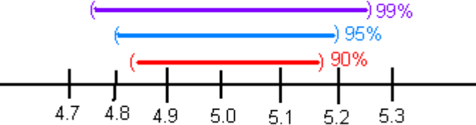
Figure 8.1: figure of Affect of Confidence Level

 

The higher level of confidence makes a wider interval. There’s a trade off between width and confidence level. You can be really confident about your answer but your answer will not be very precise. Or you can have a precise answer (small margin of error) but not be very confident about your answer.

Now look at how the sample size affects the size of the interval. Suppose figure #8.1.2 represents confidence intervals calculated on a 95% interval. A larger sample size from a representative sample makes the width of the interval nar- rower. This makes sense. Large samples are closer to the true population so the point estimate is pretty close to the true value.

Now you know everything you need to know about confidence intervals except for the actual formula. The formula depends on which parameter you are trying to estimate. With different situations you will be given the confidence interval for that parameter.

 

Homework

• Suppose you compute a confidence interval with a sample size of 25. What will happen to the confidence interval if the sample size increases to 50?

 

 

 

 

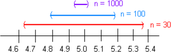
Figure 8.2: Figure of Affect of Sample Size

 

• Suppose you compute a 95% confidence interval. What will happen to the confidence interval if you increase the confidence level to 99%?
• Suppose you compute a 95% confidence interval. What will happen to the confidence interval if you decrease the confidence level to 90%?
• Suppose you compute a confidence interval with a sample size of 100. What will happen to the confidence interval if the sample size decreases to 80?
• 6353𝑘𝑚 < 𝜇 < 6384𝑘𝑚𝜇
  A 95% confidence interval is, where is the mean diameter of the Earth. State the statistical interpretation.
• 6353𝑘𝑚 < 𝜇 < 6384𝑘𝑚𝜇
  A 95% confidence interval is, where is the mean diameter of the Earth. State the real world interpretation.
• 0.52 < 𝑝 < 0.60
  In 2013, Gallup conducted a poll and found a 95% confidence interval of, where p is the proportion of Americans who believe it is the government’s responsibility for health care. Give the real world interpretation.
• 0.52 < 𝑝 < 0.60
  In 2013, Gallup conducted a poll and found a 95% confidence interval of, where p is the proportion of Americans who believe it is the government’s responsibility for health care. Give the statistical interpretation.

 

 

 

One-Sample Interval for the Proportion

Suppose you want to estimate the population proportion, p. As an example you may be curious what proportion of students at your school smoke. Or you could wonder what is the proportion of accidents caused by teenage drivers who do not have a drivers’ education class.

Confidence Interval for One Population Proportion (1-Prop Interval)

 

 

• State the random variable and the parameter in words.

x = number of successes

p = proportion of successes

• State and check the assumptions for the confidence interval
• A simple random sample of size n is taken.
• The condition for the binomial distribution are satisfied
• 𝑝̂
  𝑛 ∗ 𝑝̂ ≥ 5𝑛 ∗ 𝑞̂ ≥ 5𝑞̂ = 1 − 𝑝̂
  𝑝̂
  𝑝̂
  The sampling distribution of can be approximated by a normal dis- tributed. To determine the sampling distribution of is normally dis- tributed, you need to show thatand ,where. If this requirement is true, then the sampling distribution of is well ap- proximated by a normal curve. (In reality this is not really true, since the correct assumption deals with p. However, in a confidence interval you do not know p, so you must use 𝑝̂.)
• Find the sample statistic and the confidence interval This will be conducted using R Studio. The command is

prop.test(r, n, conf.Level=C as a decimal)

• Statistical Interpretation: In general this looks like, “you are C% confident that 𝑝̂ ± 𝐸 contains the true proportion.”
• Real World Interpretation: This is where you state what interval contains the true proportion.

 

Example:Confidence Interval for the Population Proportion

A concern was raised in Australia that the percentage of deaths of Aboriginal prisoners was higher than the percent of deaths of non-Aboriginal prisoners, which is 0.27%. A sample of six years (1990-1995) of data was collected, and it was found that out of 14,495 Aboriginal prisoners, 51 died (”Indigenous deaths in,” 1996). Find a 95% confidence interval for the proportion of Aboriginal prisoners who died.

Solution:

• State the random variable and the parameter in words.

x = number of Aboriginal prisoners who die

p = proportion of Aboriginal prisoners who die

• State and check the assumptions for the confidence interval
• A simple random sample of 14,495 Aboriginal prisoners was taken. Check: The sample was not a random sample, since it was data from six years. It

 

is the numbers for all prisoners in these six years, but the six years were not picked at random. Unless there was something special about the six years that were chosen, the sample is probably a representative sample. This assumption is probably met.

• The properties of the binomial experiment have been met. Check: There are 14,495 prisoners in this case. The prisoners are all Aboriginals, so you are not mixing Aboriginal with non-Aboriginal prisoners. There are only two outcomes, either the prisoner dies or doesn’t. The chance that one prisoner dies over another may not be constant, but if you consider all prisoners the same, then it may be close to the same probability. Thus the properties of the binomial experiment are satisfied
• bution. Check: 𝑝̂∗𝑛 =∗14495 = 51 ≥ 5 and 𝑞̂∗𝑛 =∗14495 =
  𝑝̂
  The sampling distribution ofcan be approximated with a normal distri-

51 14495−51

normal distribution.
14444 ≥ 5. The sampl1i4n4g95distribution of 𝑝̂ can be appro1x4i4m95ated with a

 

• Find the sample statistic and the confidence interval

The command in R Studio for a confidence interval for a proportion is

prop.test(51,14495, conf.level = 0.95)

 

##

## 1-sample proportions test with continuity correction ##

## data: 51 out of 14495

## X-squared = 14290, df = 1, p-value < 2.2e-16

## alternative hypothesis: true p is not equal to 0.5 ## 95 percent confidence interval:

## 0.002647440 0.004661881

## sample estimates:

##p

## 0.003518455

the 95% confidence level is 0.002647440 < 𝑝 < 0.004661881.

• Statistical Interpretation:You are 95% confident that the interval

0h.a0v0e26di<ed𝑝in<p0r.i0so0n4.7 contains the proportion of Aboriginal prisoners who

• Real World Interpretation: The proportion of Aboriginal prisoners who died in prison is between 0.26% and 0.47%.

 

Example:Confidence Interval for the Population Proportion

A researcher who is studying the effects of income levels on breastfeeding of infants hypothesizes that countries with a low income level have a different

 

 

rate of infant breastfeeding than higher income countries. It is known that in Germany, considered a high-income country by the World Bank, 22% of all babies are breastfeed. In Tajikistan, considered a low-income country by the World Bank, researchers found that in a random sample of 500 new mothers that 125 were breastfeeding their infant. Find a 90% confidence interval of the proportion of mothers in low-income countries who breastfeed their infants?

Solution:

• State you random variable and the parameter in words.

x = number of woman who breastfeed in a low-income country

p = proportion of woman who breastfeed in a low-income country

• State and check the assumptions for the confidence interval
• A simple random sample of 500 breastfeeding habits of woman in a low- income country was taken. Check: This was stated in the problem.
• The properties of a Binomial Experiment have been met. check: There were 500 women in the study. The women are considered identical, though they probably have some differences. There are only two outcomes, either the woman breastfeeds or she doesn’t. The probability of a woman breast- feeding is probably not the same for each woman, but it is probably not very different for each woman. The conditions for the binomial distribu- tion are satisfied
• tributed. Check:𝑛 ∗ 𝑝̂ = 500 ∗= 125 ≥ 5 and 𝑛 ∗ 𝑞̂ = 500 ∗=
  𝑝
  The sampling distribution ofcan be approximated with a normal dis-

125500−125

normal distribution.
375 ≥ 5, so the sampling dis5t0r0ibution of 𝑝̂ is well approximate5d00by a

 

4. Find the sample statistic and confidence interval On R studio, use the following command

prop.test(125, 500, conf.level = .90)

 

##

## 1-sample proportions test with continuity correction ##

## data: 125 out of 500

## X-squared = 124, df = 1, p-value < 2.2e-16

## alternative hypothesis: true p is not equal to 0.5 ## 90 percent confidence interval:

## 0.2185980 0.2841772

## sample estimates:

##p

## 0.25

90% confidence interval for p is 0.2185980 < 𝑝 < 0.2841772.

 

 

0.2841772
0.2185980 < 𝑝 <
4. Statistical Interpretation: You are 90% confident that

contains the proportion of women in low-income countries who breastfeed their infants.

5. Real World Interpretation: The proportion of women in low-income coun- tries who breastfeed their infants is between 0.219 and 0.284.

 

Homework

In each problem show all steps of the confidence interval. If some of the assumptions are not met, note that the results of the interval may not be correct and then continue the process of the confidence interval.

• The Arizona Republic/Morrison/Cronkite News poll published on Mon- day, October 20, 2016, found 390 of the registered voters surveyed favor Proposition 205, which would legalize marijuana for adults. The statewide telephone poll surveyed 779 registered voters between Oct. 10 and Oct. 15. (Sanchez, 2016) Find a 99% confidence interval for the proportion of Ari- zona’s who supported legalizing marijuana for adults.
• In November of 1997, Australians were asked if they thought unemploy- ment would increase. At that time 284 out of 631 said that they thought unemployment would increase (”Morgan gallup poll,” 2013). Estimate the proportion of Australians in November 1997 who believed unemployment would increase using a 95% confidence interval?
• According to the February 2008 Federal Trade Commission report on con- sumer fraud and identity theft, Arkansas had 1,601 complaints of identity theft out of 3,482 consumer complaints (”Consumer fraud and,” 2008). Calculate a 90% confidence interval for the proportion of identity theft in Arkansas.
• According to the February 2008 Federal Trade Commission report on con- sumer fraud and identity theft, Alaska had 321 complaints of identity theft out of 1,432 consumer complaints (”Consumer fraud and,” 2008). Calculate a 90% confidence interval for the proportion of identity theft in Alaska.
• In 2013, the Gallup poll asked 1,039 American adults if they believe there was a conspiracy in the assassination of President Kennedy, and found that 634 believe there was a conspiracy (”Gallup news service,” 2013). Estimate the proportion of American’s who believe in this conspiracy using a 98% confidence interval.
• In 2008, there were 507 children in Arizona out of 32,601 who were diag- nosed with Autism Spectrum Disorder (ASD) (”Autism and developmen- tal,” 2008). Find the proportion of ASD in Arizona with a confidence level of 99%.

 

 

 

One-Sample Interval for the Mean

Suppose you want to estimate the mean height of Americans, or you want to estimate the mean salary of college graduates. A confidence interval for the mean would be the way to estimate these means.

Confidence Interval for One Population Mean (t-Interval)

• State the random variable and the parameter in words. x = random variable

𝜇 = mean of random variable

• State and check the assumptions for the confidence interval
• A random sample of size n is taken.
• The population of the random variable is normally distributed, though the t-test is fairly robust to the assumption if the sample size is large. This means that if this assumption isn’t met, but your sample size is quite large, then the results of the t-test are valid.
• Find the sample statistic and confidence interval

Use R Studio to find the confidence interval. The command is

t.test(~variable, data= Data Frame, conf.level=C as a decimal)

 

• Statistical Interpretation: In general this looks like, “You are C% confident that the interval contains the true mean.”
• Real World Interpretation: This is where you state what interval contains the true mean.

How to check the assumptions of confidence interval:

In order for the confidence interval to be valid, the assumptions of the test must be true. Whenever you run a confidence interval, you must make sure the assumptions are true. You need to check them. Here is how you do this:

• For the assumption that the sample is a random sample, describe how you took the sample. Make sure your sampling technique is random.
• For the assumption that population is normal, remember the process of assessing normality from chapter 6.

 

Example:Confidence Interval for the Population Mean

A random sample of 50 body mass index (BMI) were taken from the NHANES Data frame. Estimate the mean BMI of Americans at the 95% level.

Table #8.3.1: BMI of Americans

sample_NHANES_50<-sample_n(NHANES, size=50)head(sample_NHANES_50)

 

## # A tibble: 6 x 76

##165676 2011_12 female35″ 30-39″NAWhite##252496 2009_10 female60″ 60-69″721White##369798 2011_12 female21″ 20-29″NAWhite##452326 2009_10 male28″ 20-29″343White##553524 2009_10 female39″ 30-39″471White##654437 2009_10 female51″ 50-59″619Other###… with 69 more variables: Race3 <fct>, Education <fct>,###MaritalStatus <fct>, HHIncome <fct>, HHIncomeMid <int>,###Poverty <dbl>, HomeRooms <int>, HomeOwn <fct>,###Work <fct>, Weight <dbl>, Length <dbl>, HeadCirc <dbl>,###Height <dbl>, BMI <dbl>, BMICatUnder20yrs <fct>,###BMI_WHO <fct>, Pulse <int>, BPSysAve <int>,###BPDiaAve <int>, BPSys1 <int>, BPDia1 <int>,###BPSys2 <int>, BPDia2 <int>, BPSys3 <int>, BPDia3 <int>,###Testosterone <dbl>, DirectChol <dbl>, TotChol <dbl>,###UrineVol1 <int>, UrineFlow1 <dbl>, UrineVol2 <int>,###UrineFlow2 <dbl>, Diabetes <fct>, DiabetesAge <int>,###HealthGen <fct>, DaysPhysHlthBad <int>,###DaysMentHlthBad <int>, LittleInterest <fct>,###Depressed <fct>, nPregnancies <int>, nBabies <int>,###Age1stBaby <int>, SleepHrsNight <int>,###SleepTrouble <fct>, PhysActive <fct>,###PhysActiveDays <int>, TVHrsDay <fct>, CompHrsDay <fct>,###TVHrsDayChild <int>, CompHrsDayChild <int>,###Alcohol12PlusYr <fct>, AlcoholDay <int>,###AlcoholYear <int>, SmokeNow <fct>, Smoke100 <fct>,###Smoke100n <fct>, SmokeAge <int>, Marijuana <fct>,###AgeFirstMarij <int>, RegularMarij <fct>,###AgeRegMarij <int>, HardDrugs <fct>, SexEver <fct>,###SexAge <int>, SexNumPartnLife <int>,###SexNumPartYear <int>, SameSex <fct>,###SexOrientation <fct>, PregnantNow <fct>
##ID SurveyYr GenderAge AgeDecade AgeMonths Race1 ##<int> <fct><fct> <int> <fct><int> <fct>

 

 

Solution:

• State the random variable and the parameter in words.

x = BMI of an American

𝜇 = mean BMI of Americans

• State and check the assumptions for the confidence interval
• A random sample of 50 BMI levels was taken. Check: A random sample was taken from the NHANES data frame using R Studio
• The population of BMI levels is normally distributed. Check:

gf_density(~BMI, data=sample_NHANES_50)

 

 

0.05

 

 

 

 

0.04

 

 

 

 

0.03

 

 

 

 

density
0.02

 

 

 

 

0.01

 

 

 

 

0.00

203040

BMI

 

Figure 8.3: Density Plot of BMI from NHANES sample

 

gf_qq(~BMI, data=sample_NHANES_50)

 

The density plot looks somewhat skewed right and the normal quantile plot looks somewhat linear. However, there doesn’t seem to be strong evidence that the sample comes from a population that is normally distributed. However, since the sample is moderate to large, the t-test is robust to this assumption not being met. So the results of the test are probably valid.

4. Find the sample statistic and confidence interval

 

 

 

 

 

 

 

40

 

 

 

 

 

 

 

sample
30

 

 

 

 

 

 

 

20

 

 

 

 

 

−2−1012

theoretical

 

Figure 8.4: Normal Quantile Plot of BMI from NHANES sample

 

On R Studio, the command would be

t.test(~BMI, data= sample_NHANES_50, conf.level=0.95)

 

##

## One Sample t-test ##

## data: BMI

## t = 25.818, df = 48, p-value < 2.2e-16

## alternative hypothesis: true mean is not equal to 0 ## 95 percent confidence interval:

## 25.08079 29.31717

## sample estimates:

## mean of x ## 27.19898

The sample statistic is the mean of x in the output, and confidence interval is under the words 95 percent confidence interval.

4. Statistical Interpretation: You are 95% confident that 24.87190 < 𝜇 < 28.71422 contains the mean BMI of Americans.

5. Real World Interpretation: The mean BMI of Americans is between 24.87 and 28.71 𝑘𝑔/𝑚2.

 

 

𝑘𝑔/𝑚
Notice that in example #7.3.2, you were asked if the mean BMI of Americans was different from Australians’ mean BMI of 27.22. The interval that example #8.3.1 calculated does contain the value of 27.2. So you can’t say that Americans’ mean BMI and Australians’ mean BMI are different.This means that you can just use confidence intervals and not conduct hypothesis tests at all if you prefer.

 

Example:Confidence Interval for the Population Mean

The data in table #8.3.2 are the life expectancies for all people in European countries (”WHO life expectancy,” 2013). Table #8.3.3 filtered the data frame for just males and just year 2000. The year 2000 was randomly chosen as the year to use. Estimate the mean life expectancy for a man in Europe at the 99% level.

Table #8.3.2: Life Expectancies for European Countries

Expectancy<-read.csv( “https://krkozak.github.io/MAT160/Life_expectancy_Europe.csv”)head(Expectancy)

 

##	year	WHO_region country	sex	expect
##	1 1990	Europe Albania	Male	67
##	2 1990	Europe Albania	Female	71
##	3 1990	Europe Albania	Both sexes	69
##	4 2000	Europe Albania	Male	68
##	5 2000	Europe Albania	Female	73
##	6 2000	Europe Albania	Both sexes	71

Table #8.3.3: Life Expectancies of males in European Countries in 2000

Expectancy_male<- Expectancy%>%filter(sex==”Male”, year==”2000″)head(Expectancy_male)

##year WHO_regioncountry sex expect

## 1 2000	EuropeAlbania Male	68
## 2 2000	EuropeAndorra Male	76
## 3 2000	EuropeArmenia Male	68
## 4 2000	EuropeAustria Male	75
## 5 2000	Europe Azerbaijan Male	64
## 6 2000	EuropeBelarus Male	63

Code book for data frame Expectancy See example 7.3.3 in Section 7.3

Solution:

 

 

• State the random variable and the parameter in words.

x = life expectancy for a European man

𝜇 = mean life expectancy for European men

• State and check the assumptions for the confidence interval
• A random sample of 53 life expectancies of European men in 2000 was taken. Check: The data is actually all of the life expectancies for every country that is considered part of Europe by the World Health Organiza- tion in the year 2000. Since the year 2000 was picked at random, then the sample is a random sample.
• The distribution of life expectancies of European men in 2000 is normally distributed. Check:

gf_density(~expect, data=Expectancy_male)

 

 

 

 

 

 

 

 

0.06

 

 

 

 

 

density
0.04

 

 

 

 

 

0.02

 

 

 

 

 

0.00

60657075

expect

 

Figure 8.5: (ref:expactancy-male8-density-cap)

 

gf_qq(~expect, data=Expectancy_male)

 

This sample does not appear to come from a population that is normally dis- tributed. This sample is moderate to large, so it is good that the t-test is robust.

• Find the sample statistic and confidence interval

 

 

 

 

 

 

 

75

 

 

 

 

 

sample
70

 

 

 

 

 

65

 

 

 

 

 

60

 

 

 

−2−1012

theoretical

 

Figure 8.6: Normal Quntile Plot of Life Expectancies of Males in Europe in 2000

 

On R Studio, the command would be

t.test(~expect, data=Expectancy_male, conf.level=0.99)

 

##

## One Sample t-test ##

## data: expect

## t = 90.919, df = 52, p-value < 2.2e-16

## alternative hypothesis: true mean is not equal to 0 ## 99 percent confidence interval:

## 68.60071 72.75778

## sample estimates:

## mean of x ## 70.67925

Sample statistic is 70.68 years, and the confidence interval is 68.60071 < 𝜇 < 72.75778.

• Statistical Interpretation: You are 99% confident that 68.60071 < 𝜇 < 72.75778 contains the mean life expectancy of European men.
• Real World Interpretation: The mean life expectancy of European men is

 

between 68.60 and 72.76 years.

 

Homework

** In each problem show all steps of the confidence interval. If some of the assumptions are not met, note that the results of the interval may not be correct and then continue the process of the confidence interval.**

• The Kyoto Protocol was signed in 1997, and required countries to start re- ducing their carbon emissions. The protocol became enforceable in Febru- ary 2005. Table 8.3.4 contains a random sample of CO2 emissions in 2010 (CO2 emissions (metric tons per capita), 2018). Find a 99% confidence interval for the mean CO-2 emissions in 2010.

Table #8.3.4: CO2 Emissions (in metric tons per capita) in 2010

Emission <- read.csv( “https://krkozak.github.io/MAT160/CO2_emission.csv”)head(Emission)

 

##	country		y1960		y1961		y1962		y1963
##	1	Aruba	NA		NA		NA		NA
##	2	Afghanistan	0.04605671		0.05358884		0.07372083		0.07416072
##	3	Angola	0.10083534		0.08220380		0.21053148		0.20273730
##	4	Albania	1.25819493		1.37418605		1.43995596		1.18168114
##	5	Andorra	NA		NA		NA		NA
##	6	Arab World	0.64573587		0.68746538		0.76357363		0.87823769
##		y1964	y1965		y1966		y1967		y1968
##	1	NA	NA	NA		NA		NA
##	2	0.08617361	0.1012849	0.1073989		0.1234095		0.1151425
##	3	0.21356035	0.2058909	0.2689414		0.1721017		0.2897181
##	4	1.11174196	1.1660990	1.3330555		1.3637463		1.5195513
##	5	NA	NA	NA		NA		NA
##	6	1.00305335	1.1705403	1.2781736		1.3374436		1.5522420
##		y1969	y1970	y1971		y1972		y1973
##	1	NA	NA	NA		NA		NA
##	2	0.08650986	0.1496515	0.1652083		0.1299956		0.1353666
##	3	0.48023402	0.6082236	0.5645482		0.7212460		0.7512399
##	4	1.55896757	1.7532399	1.9894979		2.5159144		2.3038974
##	5	NA	NA	NA		NA		NA
##	6	1.79866893	1.8103078	2.0037220		2.1208746		2.4095329
##		y1974y1975y1976y1977y1978
##	1	NANANANANA
##	2	0.1545032 0.1676124 0.1535579 0.1815222 0.1618942
##	3	0.7207764 0.6285689 0.4513535 0.4692212 0.6947369
##	4	1.8490067 1.9106336 2.0135846 2.2758764 2.5306250
##	5	NANANANANA
##	6	2.2858907 2.1967827 2.5843424 2.6487624 2.7623331

 

 

##	y1979		y1980		y1981		y1982		y1983
##	1	NA	NA		NA		NA		NA
##	2	0.1670664	0.1317829		0.1506147		0.1631039		0.2012243
##	3	0.6830629	0.6409664		0.6111351		0.5193546		0.5513486
##	4	2.8982085	1.9350583		2.6930239		2.6248568		2.6832399
##	5	NA	NA		NA		NA		NA
##	6	2.8636143	3.0928915		2.9302350		2.7231544		2.8165670
##		y1984	y1985		y1986		y1987		y1988
##	1	NA	NA		2.8683194		7.2351980		10.0261792
##	2	0.2319613	0.2939569		0.2677719		0.2692296		0.2468233
##	3	0.5209829	0.4719028		0.4516189		0.5440851		0.4635083
##	4	2.6942914	2.6580154		2.6653562		2.4140608		2.3315985
##	5	NA	NA		NA		NA		NA
##	6	2.9813539	3.0618504		3.2844996		3.1978064		3.2950428
##	y1989		y1990			y1991			y1992	y1993
##	1	10.6347326	26.3745032 26.0461298 21.44255880 22.00078616
##	2	0.2338822	0.2106434 0.1833636 0.09619658 0.08508711
##	3	0.4372955	0.4317436 0.4155308 0.41052293 0.44172110
##	4	2.7832431	1.6781067 1.3122126 0.77472491 0.72379029
##	5	NA	7.4673357 7.1824566 6.91205339 6.73605485
##	6	3.2566742	3.0169588 3.2366449 3.41548491 3.66944563
##	y1994			y1995		y1996			y1997
##	1	21.03624511		20.77193616		20.31835337		20.42681771
##	2	0.07580649		0.06863986		0.06243461		0.05664234
##	3	0.28811907		0.78703255		0.72623346		0.49636125
##	4	0.60020371		0.65453713		0.63662531		0.49036506
##	5	6.49420042		6.66205168		7.06507147		7.23971272
##	6	3.67435821		3.42400952		3.32830368		3.14553220
##		y1998		y1999		y2000		y2001
##	1	20.58766915		20.31156677		26.19487524		25.93402441
##	2	0.05276322		0.04072254		0.03723478		0.03784614
##	3	0.47581516		0.57708291		0.58196150		0.57431605
##	4	0.56027144		0.96016441		0.97817468		1.05330418
##	5	7.66078389		7.97545440		8.01928429		7.78695000
##	6	3.34996719		3.32834106		3.70385708		3.60795615
##		y2002		y2003		y2004		y2005
##	1	25.67116178		26.42045209		26.51729342		27.20070778
##	2	0.04737732		0.05048134		0.03841004		0.05174397
##	3	0.72295888		0.50022540		1.00187812		0.98573636
##	4	1.22954071		1.41269720		1.37621273		1.41249821
##	5	7.59061514		7.31576071		7.35862494		7.29987194
##	6	3.60461275		3.79646741		4.06856241		4.18567731
##		y2006		y2007		y2008		y2009		y2010
##	1	26.94772597		27.89502282		26.2295527 25.9153221 24.6705289
##	2	0.06242753		0.08389281		0.1517209 0.2383985 0.2899876
##	3	1.10501903		1.20313400		1.1850005 1.2344251 1.2440915

 

 

##	4	1.30257637 1.32233486			1.4843111		1.4956002		1.5785736
##	5	6.74605213 6.51938706			6.4278100		6.1215799		6.1225947
##	6	4.28571918 4.11714755			4.4089483		4.5620151		4.6368134
##		y2011y2012			y2013		y2014 y2015		y2016
##	1	24.5075162	13.1577223	8.353561		8.4100642		NA	NA
##	2	0.4064242	0.3451488	0.310341		0.2939464		NA	NA
##	3	1.2526808	1.3302186	1.253776		1.2903068		NA	NA
##	4	1.8037147	1.6929083	1.749211		1.9787633		NA	NA
##	5	5.8674102	5.9168840	5.901775		5.8329062		NA	NA
##	6	4.5594617	4.8377796	4.674925		4.8869875		NA	NA

 

 

 

 

 

 

 

##y2017 y2018##1NANA##2NANA##3NANA##4NANA##5NANA##6NANA
Code book for data frame Emission See Homework problem 7.3.1 in section 7.3

• The amount of sugar in a Krispy Kream glazed donut is 10 g. Many people feel that cereal is a healthier alternative for children over glazed donuts. Table #8.3.5 contains the amount of sugar in a sample of cereal that is geared towards children (breakfast cereal, 2019). Estimate the mean amount of sugar in children’s cereal at the 95% confidence level.

Table #8.3.5: Nutrition Amounts in Cereal

Sugar <- read.csv( “https://krkozak.github.io/MAT160/cereal.csv”)head(Sugar)

 

##		namemanfage type
##	1	100%_BranNabisco adult cold
##	2	100%_Natural_BranQuaker_Oats adult cold
##	3	All-BranKelloggs adult cold
##	4	All-Bran_with_Extra_FiberKelloggs adult cold
##	5	Almond_Delight Ralston_Purina adult cold
##	6	Apple_Cinnamon_Cheerios General_Mills child cold
##		colories protein fat sodium fiber carb sugar shelf
##	1	70	4	1130 10.0 5.0	6	3
##	2	120	3	5152.0 8.0	8	3
##	3	70	4	12609.0 7.0	5	3
##	4	50	4	0140 14.0 8.0	0	3
##	5	110	2	22001.0 14.0	8	3
##	6	110	2	21801.5 10.5	10	1

##potassium vit weight serving

 

 

##	1	280	25	1	0.33
##	2	135	0	1	-1.00
##	3	320	25	1	0.33
##	4	330	25	1	0.50
##	5	-1	25	1	0.75
##	6	70	25	1	0.75

Code book for data frame Sugar See Homework problem 7.3.2 in section 7.3

A new data frame will need to be created of just cereal for children. To create that use the following command in R Studio

Table #8.3.6: Nutrition Amounts in Children’s Cereal

Sugar_chidren<- Sugar%>%filter(age==”child”) head(Sugar_chidren)

 

##name manf age type ## 1 Apple_Cinnamon_Cheerios General_Mills child cold ## 2Apple_Jacks Kelloggs child cold

## 3Bran_Chex Ralston_Purina child cold

## 4 Cap’n’Crunch Quaker_Oats child cold

## 5Cheerios General_Mills child cold ## 6 Cinnamon_Toast_Crunch General_Mills child cold ## colories protein fat sodium fiber carb sugar shelf

## 1	110	2	2	180	1.5 10.5	10	1
## 2	110	2	0	125	1.0 11.0	14	2
## 3	90	2	1	200	4.0 15.0	6	1
## 4	120	1	2	220	0.0 12.0	12	2
## 5	110	6	2	290	2.0 17.0	1	1
## 6	120	1	3	210	0.0 13.0	9	2

##1702510.75##2302511.00##31252510.67##4352510.75##51052511.25##6452510.75
## potassium vit weight serving

 

 

 

 

 

 

• The FDA regulates that fish that is consumed is allowed to contain 1.0 mg/kg of mercury. In Florida, bass fish were collected in 53 different lakes to measure the health of the lakes. The data frame of measurements from Florida lakes is in table #8.3.7 (NISER 081107 ID Data, 2019). Calculate with 90% confidence the mean amount of mercury in fish in Florida lakes. Is there too much mercury in the fish in Florida?

##pulse_beforepulse_afteryear##1707193##2807693##36812595##4706895##5928496

Table #8.3.7: Health of Florida lake Fish

Mercury<- read.csv( “https://krkozak.github.io/MAT160/mercury.csv”)head(Mercury)

 

##	ID	lake	alkalinity		ph	calcium	chlorophyll
##	1 1	Alligator	5.9		6.1	3.0	0.7
##	2 2	Annie	3.5		5.1	1.9	3.2
##	3 3	Apopka	116.0		9.1	44.1	128.3
##	4 4	Blue_Cypress	39.4		6.9	16.4	3.5
##	5 5	Brick	2.5		4.6	2.9	1.8
##	6 6	Bryant	19.6		7.3	4.5	44.1
##mercury no.samples min max X3_yr_standmercury age_data
##	11.23		5	0.85 1.43	1.53			1
##	21.33		7	0.92 1.90	1.33			0
##	30.04		6	0.04 0.06	0.04			0
##	40.44		12	0.13 0.84	0.44			0
##	51.20		12	0.69 1.50	1.33			1
##	60.27		14	0.04 0.48	0.25			1

Code book for data frame Mercury See Homework problem 7.3.3 in section 7.3

• The data frame Pulse (Table 8.3.8) contains various variables about a person including their pulse rates before the subject exercised and after the subject ran in place for one minute. Estimate the mean pulse rate of females who do drink alcohol with a 95% level of confidence?

Table #8.3.8: Pulse Rates Pulse Rates of people Before and After Exercise

Pulse<-read.csv( “https://krkozak.github.io/MAT160/pulse.csv”)head(Pulse)

##height weight age gender smokes alcohol exercise ran

## 1	170	68	22	male	yes	yes moderate sat
## 2	182	75	26	male	yes	yes moderate sat
## 3	180	85	19	male	yes	yes moderate ran
## 4	182	85	20	male	yes	yes	low sat
## 5	167	70	22	male	yes	yes	low sat
## 6	178	86	21	male	yes	yes	low sat

 

 

## 6 76 80 98

Code book for data frame Pulse, see homework problem 3.2.5 in section 3.2

To create a new data frame with just females who drink alcohol use the following command, where the new name is Females: Table #8.3.9: Pulse Rates Pulse Rates of people Before and After Exercise

Females<- Pulse%>%filter(gender==”female”, alcohol==”yes”)head(Females)

##height weight age gender smokes alcohol exercise ran

##	1	165	60	19	female	yes	yes	low	ran
##	2	163	47	23	female	yes	yes	low	ran
##	3	173	57	18	female	no	yes	moderate	sat
##	4	179	58	19	female	no	yes	moderate	ran
##	5	167	62	18	female	no	yes	high	ran
##	6	173	64	18	female	no	yes	low	sat
##		pulse_before		pulse_after		year
##	1	88		120		98
##	2	71		125		98
##	3	86		88		93
##	4	82		150		93
##	5	96		176		93
##	6	90		88		93

• The economic dynamism is an index of productive growth in dollars. Eco- nomic data for many countries are in table #8.3.10 (SOCR Data 2008 World CountriesRankings, 2019).

##10LowalAlbaniaSmallSouthern_Europe popS##21MiddledzAlgeriaMediumNorth_Africa popM##32MiddlearArgentinaMediumSouth_America popM##43HighauAustraliaMediumAustralia popM##54HighatAustriaSmallCentral_Europe popS##65LowazAzerbaijanSmallcentral_Asia popS##EDEduHIQOLPE OA Relig##134.0862 81.016471.0244 67.9240 58.6742 5739##225.8057 74.802766.1951 60.9347 32.6054 8595
Table #8.3.10: Economic Data for Countries

Economics <- read.csv( “https://krkozak.github.io/MAT160/Economics_country.csv”)head(Economics)

##Id incGroup keyname popGroupregion key2

 

 

##	3	37.4511	69.8825	78.2683	68.1559	68.6647	46	66
##	4	71.4888	91.4802	95.1707	90.5729	90.9629	4	65
##	5	53.9431	90.4578	90.3415	87.5630	91.2073	18	20
##	6	53.6457	68.9880	58.9512	68.9572	40.0390	69	50

Code book for data frame Economics See Homework problem 7.3.5 in section 7.3

Create a data frame that contains only middle income countries. Find a 95% confidence interval for the mean econimic dynamism for middle income coun- tries. To create a new data frame with just middle income countries use the fol- lowing command, where the new name is Middle_economics: Table #8.3.11: Economic Data for Middle income Countries

Middle_economics<- Economics%>%filter(incGroup==”Middle”) head(Middle_economics)

##Id incGroup keyname popGroupregion key2

##	1	1	Middle		dz	Algeria		Medium		North_Africa			popM
##	2	2	Middle		ar	Argentina		Medium		South_America			popM
##	3	7	Middle		by	Belarus		Small		central_Asia			popS
##	4	10	Middle		bw	Botswana		Small		Africa			popS
##	5	11	Middle		br	Brazil		Large		South_America			popL
##	6	12	Middle		bg	Bulgaria		Small		Southern_Europe			popS
##			ED		Edu	HI		QOL		PE OA Relig
##	1	25.8057		74.8027		66.1951	60.9347		32.6054		85	95
##	2	37.4511		69.8825		78.2683	68.1559		68.6647		46	66
##	3	51.9150		86.6155		66.1951	74.1467		34.0501		56	34
##	4	43.6952		73.4608		34.8049	50.0875		72.6833		80	80
##	5	47.8506		71.3735		71.0244	62.4238		67.4131		48	87
##	6	43.7178		82.2277		75.8537	73.1197		73.1686		38	50

• Table #8.3.12 contains the percentage of woman receiving prenatal care in a sample of countries over several years. (births per woman), 2019). Estimate the average percentage of women receiving prenatal care in 2009 (p2009) with a 95% confidence interval?

## 1AngolaAGOSub-Saharan Africa## 2ArmeniaARMEurope & Central Asia## 3BelizeBLZLatin America & Caribbean
Table #8.3.12: Data of Prenatal Care versus Health Expenditure

Fert_prenatal<- read.csv( “https://krkozak.github.io/MAT160/fertility_prenatal.csv”)head(Fert_prenatal)

##Country.Name Country.CodeRegion

 

## 4 Cote d’IvoireCIVSub-Saharan Africa## 5EthiopiaETHSub-Saharan Africa## 6GuineaGINSub-Saharan Africa
##IncomeGroupf1960f1961f1962f1963f1964f1965##1Lowermiddleincome7.4787.5247.5637.5927.6117.619##2Uppermiddleincome4.7864.6704.5214.3454.1503.950##3Uppermiddleincome6.5006.4806.4606.4406.4206.400##4Lowermiddleincome7.6917.7207.7507.7817.8117.841##5Lowincome6.8806.8776.8756.8726.8676.864##6Lowincome6.1146.1276.1386.1476.1546.160

 

 

 

 

 

 

 

 

 

 

##	f1966		f1967	f1968	f1969	f1970	f1971	f1972	f1973	f1974
##	1	7.618	7.613	7.608	7.604	7.601	7.603	7.606	7.611	7.614
##	2	3.758	3.582	3.429	3.302	3.199	3.114	3.035	2.956	2.875
##	3	6.379	6.358	6.337	6.316	6.299	6.288	6.284	6.285	6.287
##	4	7.868	7.893	7.912	7.927	7.936	7.941	7.942	7.939	7.929
##	5	6.867	6.880	6.903	6.937	6.978	7.020	7.060	7.094	7.121
##	6	6.168	6.177	6.189	6.205	6.225	6.249	6.277	6.306	6.337
##		f1975	f1976	f1977	f1978	f1979	f1980	f1981	f1982	f1983
##	1	7.615	7.609	7.594	7.571	7.540	7.504	7.469	7.438	7.413
##	2	2.792	2.712	2.641	2.582	2.538	2.510	2.499	2.503	2.517
##	3	6.278	6.250	6.195	6.109	5.992	5.849	5.684	5.510	5.336
##	4	7.910	7.877	7.828	7.763	7.682	7.590	7.488	7.383	7.278
##	5	7.143	7.167	7.195	7.230	7.271	7.316	7.360	7.397	7.424
##	6	6.369	6.402	6.436	6.468	6.500	6.529	6.557	6.581	6.602
##		f1984	f1985	f1986	f1987	f1988	f1989	f1990	f1991	f1992
##	1	7.394	7.380	7.366	7.349	7.324	7.291	7.247	7.193	7.130
##	2	2.538	2.559	2.578	2.591	2.592	2.578	2.544	2.484	2.400
##	3	5.170	5.019	4.886	4.771	4.671	4.584	4.508	4.436	4.363
##	4	7.176	7.078	6.984	6.892	6.801	6.710	6.622	6.536	6.454
##	5	7.437	7.435	7.418	7.387	7.347	7.298	7.246	7.193	7.143
##	6	6.619	6.631	6.637	6.637	6.631	6.618	6.598	6.570	6.535
##		f1993	f1994	f1995	f1996	f1997	f1998	f1999	f2000	f2001
##	1	7.063	6.992	6.922	6.854	6.791	6.734	6.683	6.639	6.602
##	2	2.297	2.179	2.056	1.938	1.832	1.747	1.685	1.648	1.635
##	3	4.286	4.201	4.109	4.010	3.908	3.805	3.703	3.600	3.496
##	4	6.374	6.298	6.224	6.152	6.079	6.006	5.932	5.859	5.787
##	5	7.094	7.046	6.995	6.935	6.861	6.769	6.659	6.529	6.380
##	6	6.493	6.444	6.391	6.334	6.273	6.211	6.147	6.082	6.015
##		f2002	f2003	f2004	f2005	f2006	f2007	f2008	f2009	f2010
##	1	6.568	6.536	6.502	6.465	6.420	6.368	6.307	6.238	6.162
##	2	1.637	1.648	1.665	1.681	1.694	1.702	1.706	1.703	1.693
##	3	3.390	3.282	3.175	3.072	2.977	2.893	2.821	2.762	2.715
##	4	5.717	5.651	5.589	5.531	5.476	5.423	5.372	5.321	5.269
##	5	6.216	6.044	5.867	5.690	5.519	5.355	5.201	5.057	4.924
##	6	5.947	5.877	5.804	5.729	5.653	5.575	5.496	5.417	5.336
##		f2011	f2012	f2013	f2014	f2015	f2016	f2017	p1986	p1987

 

## 1NANANANANANANANANA## 2NANANANANANANANANA## 3NANANA96NANANANANA## 4NANANANANANA83.2NANA## 5NANANANANANANANANA## 6NANANANA57.6NANANANA

##	1	6.082	6.000	5.920	5.841	5.766	5.694	5.623	NA	NA
##	2	1.680	1.664	1.648	1.634	1.622	1.612	1.604	NA	NA
##	3	2.676	2.642	2.610	2.578	2.544	2.510	2.475	NA	NA
##	4	5.216	5.160	5.101	5.039	4.976	4.911	4.846	NA	NA
##	5	4.798	4.677	4.556	4.437	4.317	4.198	4.081	NA	NA
##	6	5.256	5.175	5.094	5.014	4.934	4.855	4.777	NA	NA
##		p1988	p1989	p1990	p1991	p1992	p1993	p1994	p1995	p1996

 

 

 

 

 

 

##	p1997		p1998		p1999	p2000	p2001		p2002		p2003	p2004		p2005
##	1	NA	NA		NA	NA	65.6		NA		NA	NA		NA
##	2	82	NA		NA	92.4	NA		NA		NA	NA		93.0
##	3	NA	98		95.9	100.0	NA		98		NA	NA		94.0
##	4	NA	NA		84.3	87.6	NA		NA		NA	NA		87.3
##	5	NA	NA		NA	26.7	NA		NA		NA	NA		27.6
##	6	NA	NA		70.7	NA	NA		NA		84.3	NA		82.2
##		p2006	p2007		p2008	p2009	p2010		p2011		p2012	p2013		p2014
##	1	NA	79.8		NA	NA	NA		NA		NA	NA		NA
##	2	NA	NA		NA	NA	99.1		NA		NA	NA		NA
##	3	94.0	99.2		NA	NA	NA		96.2		NA	NA		NA
##	4	84.8	NA		NA	NA	NA		NA		90.6	NA		NA
##	5	NA	NA		NA	NA	NA		33.9		NA	NA		41.2
##	6	NA	88.4		NA	NA	NA		NA		85.2	NA		NA
##	p2015		p2016		p2017	p2018	e2000				e2001	e2002
##	1	NA	81.6		NA	NA	2.334435			5.483824		4.072288
##	2	NA	99.6		NA	NA	6.505224			6.536262		5.690812
##	3	97.2	97.2		NA	NA	3.942030			4.228792		3.864327
##	4	NA	93.2		NA	NA	5.672228			4.850694		4.476869
##	5	NA	62.4		NA	NA	4.365290			4.713670		4.705820
##	6	NA	84.3		NA	NA	3.697726			3.884610		4.384152
##	e2003				e2004	e2005			e2006		e2007			e2008
##	1	4.454100		4.757211		3.734836		3.366183			3.211438		3.495036
##	2	5.610725		8.227844		7.034880		5.588461			5.445144		4.346749
##	3	4.260178		4.091610		4.216728		4.163924			4.568384		4.646109
##	4	4.645306		5.213588		5.353556		5.808850			6.259154		6.121604
##	5	4.885341		4.304562		4.100981		4.226696			4.801925		4.280639
##	6	3.651081		3.365547		2.949490		2.960601			3.013074		2.762090
##		e2009		e2010		e2011		e2012			e2013		e2014
##	1	3.578677		2.736684		2.840603		2.692890			2.990929		2.798719
##	2	4.689046		5.264181		3.777260		6.711859			8.269840		10.178299
##	3	5.311070		5.764874		5.575126		5.322589			5.727331		5.652458
##	4	6.223329		6.146566		5.978840		6.019660			5.074942		5.043462

 

 

## 5	4.412473 5.466372 4.468978 4.539596 4.075065 4.033651
## 6	2.936868 3.067742 3.789550 3.503983 3.461137 4.780977
##	e2015e2016
## 1	2.950431 2.877825
## 2	10.117628 9.927321
## 3	5.884248 6.121374
## 4	5.262711 4.403621
## 5	3.975932 3.974016
## 6	5.827122 5.478273

Code book for Data frame Fert_prenatal See Problem 2.3.4 in Section

2.3 homework

• Maintaining your balance may get harder as you grow older. A study was conducted to see how steady the elderly is on their feet. They had the subjects stand on a force platform and have them react to a noise. The force platform then measured how much they swayed forward and backward, and the data is in table #8.3.13 (Maintaining Balance while Concentrating, 2019). Find the mean forward/backward sway of elderly person? Use a 95% confidence level. Follow the filtering methods in other homework problems to create a data frame for only Elderly.

Table #8.3.13: Sway (in mm) of Elderly Subjects

Sway <- read.csv( “https://krkozak.github.io/MAT160/sway.csv”)head(Sway)

##age fbsway sidesway

## 1 Elderly	19	14
## 2 Elderly	30	41
## 3 Elderly	20	18
## 4 Elderly	19	11
## 5 Elderly	29	16
## 6 Elderly	25	24

Code book for data frame Sway See Homework problem 7.3.7 in section 7.3

 

 

 

Data Sources:

Australian Human Rights Commission, (1996). Indigenous deaths in custody 1989 – 1996. Retrieved from website: http://www.humanrights.gov.au/ publications/indigenous-deaths-custody

CDC features – new data on autism spectrum disorders. (2013, November 26). Retrieved from http://www.cdc.gov/features/countingautism/

Center for Disease Control and Prevention, Prevalence of Autism Spectrum

 

 

Disorders – Autism and Developmental Disabilities Monitoring Network. (2008). Autism and developmental disabilities monitoring network-2012. Retrieved from website: http://www.cdc.gov/ncbddd/autism/documents/ADDM-2012- Community-Report.pdf

Federal Trade Commission, (2008). Consumer fraud and identity theft complaint data: January-December 2007. Retrieved from website: http://www.ftc.gov/ opa/2008/02/fraud.pdf

Sanchez, Y. W. (2016, October 20). Poll: Arizona voters still favor legal- izing marijuana.Retrieved from https://www.azcentral.com/story/news/ politics/elections/2016/10/20/poll-arizona-marijuana-legalization-proposition- 205/92417690/

http://apps.who.int/gho/athena/data/download.xsl?format=xml&target= GHO/WHOSIS_000001&profile=excel&filter=COUNTRY:;SEX:;REGION:EUR

CO2 emissions (metric tons per capita). (n.d.). Retrieved July 18, 2019, from https://data.worldbank.org/indicator/EN.ATM.CO2E.PC

(n.d.). Retrieved July 18, 2019, from https://www.idvbook.com/teaching- aid/data-sets/the-breakfast-cereal-data-set/ The Best Kids’ Cereal. (n.d.). Retrieved July 18, 2019, from https://www.ranker.com/list/best-kids- cereal/ranker-food

Lange TL, Royals HE, Connor LL (1993) Influence of water chemistry on mer- cury concentration in largemouth bass from Florida lakes. Trans Am Fish Soc 122:74-84. Michael K. Saiki, Darell G. Slotton, Thomas W. May, Shaun M. Ay- ers, and Charles N. Alpers (2000) Summary of Total Mercury Concentrations in Fillets of Selected Sport Fishes Collected during 2000–2003 from Lake Natoma, Sacramento County, California (Raw data is included in appendix), U.S. Geo- logical Survey Data Series 103, 1-21. NISER 081107 ID Data. (n.d.). Retrieved July 18, 2019, from http://wiki.stat.ucla.edu/socr/index.php/NISER_081107_ ID_Data

SOCR Data 2008 World CountriesRankings.(n.d.).Retrieved July 19, 2019,fromhttp://wiki.stat.ucla.edu/socr/index.php/SOCR_Data_2008_ World_CountriesRankings#SOCR_Data_-_Ranking_of_the_top_100_ Countries_based_on_Political.2C_Economic.2C_Health.2C_and_Quality-

of-Life_Factors

Maintaining Balance while Concentrating. (n.d.). Retrieved July 19, 2019, from http://www.statsci.org/data/general/balaconc.html

 

 

 

 

 

Chapter 9