9.2 Measures of Variation
Applications
Back to our Bull Trout! Let's pull two samples of five fish from two different populations, one in the Bull River and the other population in the Clark Fork River.
| Bull River | Bull River | Clark Fork River | Clark Fork River | |
| 225 | 301 | 980 | 1023 | |
| 335 | 175 | 35 | 22 | |
| 220 | 208 | 23 | 30 | |
| 130 | 306 | 25 | 21 | |
| 154 | 108 | 40 | 21 | |
| mean | 212.8 | 219.6 | 220.6 | 223.4 |
What is the mean of each sample? Do you feel like this adequately describes the sample? What is different about samples from these two populations? How can we communicate this difference?
Normal Distributions & Standard Deviation
A normal distribution, often referred to as a bell curve, is symmetrical on the left and right, with the mean, median, and mode being the value in the center. There are lots of data values near the center, then fewer and fewer as the values get further from the center. A normal distribution describes the data in many real-world situations.
One of the best ways to demonstrate the normal distribution is to drop balls through a board of evenly spaced pegs, as shown here. (The Plinko game on The Price Is Right is a well known example of this.) Each time a ball hits a peg, it has a fifty-fifty chance of going left or right. For most balls, the number of lefts and rights are roughly equal, and the ball lands near the center. Only a few balls have an extremely lopsided number of lefts and rights, so there are not many balls at either end. As you can see, the distribution is not perfect, but it is approximated by the normal curve drawn on the glass.

The standard deviation is a measure of the spread of the data: data with lots of results close to the mean has a smaller standard deviation, and data with results spaced further from the mean has a larger standard deviation. The standard deviation is a measuring stick for a particular set of data.
The 68-95-99.7 Rule
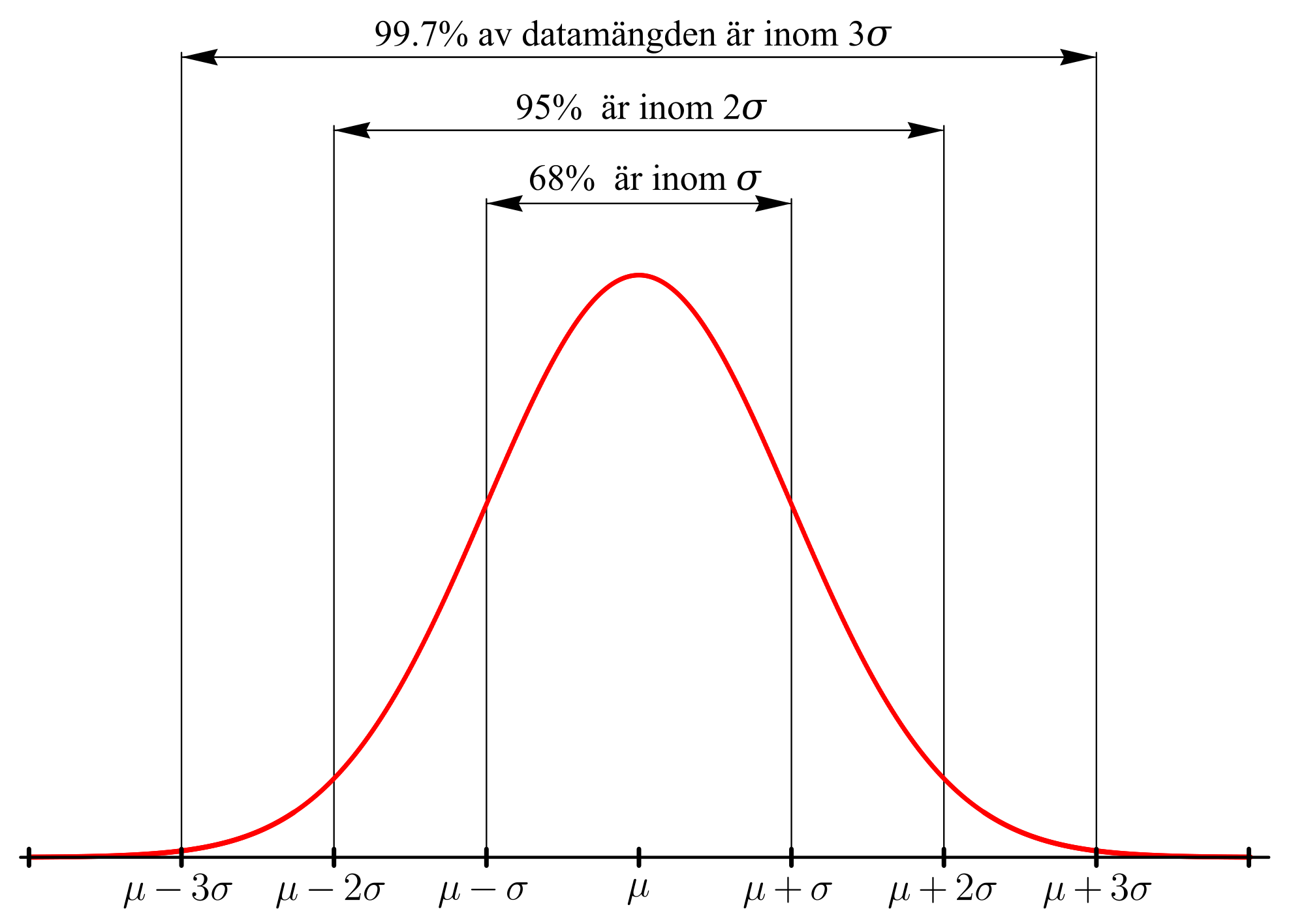
The 68-95-99.7 rule: In a normal distribution, approximately...
- [latex]68\%[/latex] of the numbers are within [latex]1[/latex] standard deviation above or below the mean
- [latex]95\%[/latex] of the numbers are within [latex]2[/latex] standard deviations above or below the mean
- [latex]99.7\%[/latex] of the numbers are within [latex]3[/latex] standard deviations above or below the mean
This is an empirical rule because it is based on observation of how the world works, rather than being based on a formula.[1]
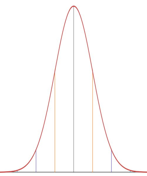
Returning to the ball-dropping experiment, let's assume that the standard deviation is three columns wide.[2] In the picture below, the green line marks the center of the distribution.
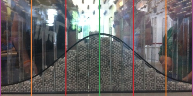
First, the two red lines are each three columns away from the center, which is one standard deviation above and below the center, so about 68% of the balls will land between the red lines.
Next, the two orange lines are another three columns farther away from the center, which is six columns or two standard deviations above and below the center, so about 95% of the balls will land between the orange lines.
And finally, the two purple lines are another three columns farther away from the center, which is nine columns or three standard deviations above and below the center, so about 99.7% of the balls will land between the purple lines. We can expect that [latex]997[latex] out of [latex]1,000[latex] balls will land between the purple lines, leaving only [latex]3[latex] out of [latex]1,000[latex] landing beyond the purple lines on either end.
Okay, that was a lot of information. For our purposes, the following restatement of the 68-95-99.7 rule may be more practical.
- [latex]68\%[/latex] of the numbers are between [latex]\mu-\sigma[/latex] and [latex]\mu+\sigma[/latex]
- [latex]95\%[/latex] of the numbers are between [latex]\mu-2\sigma[/latex] and [latex]\mu+2\sigma[/latex]
- [latex]99.7\%[/latex] of the numbers are between [latex]\mu-3\sigma[/latex] and [latex]\mu+3\sigma[/latex]
Practice Exercises
The heights of U.S. females are normally distributed. The average height is around [latex]63.5[/latex] inches ([latex]5[/latex] ft [latex]3.5[/latex] in) and the standard deviation is [latex]3[/latex] inches. Use the 68-95-99.7 rule to fill in the blanks.
- About [latex]68\%[/latex] of the women should be between _______ and _______ inches tall.
- About [latex]95\%[/latex] of the women should be between _______ and _______ inches tall.
- About [latex]99.7\%[/latex] of the women should be between _______ and _______ inches tall.
The heights of U.S. males are normally distributed. The average height is around [latex]69.5[latex] inches ([latex]5[latex] ft [latex]9.5[latex] in) and the standard deviation is [latex]3[latex] inches. Use the 68-95-99.7 rule to fill in the blanks.
- About [latex]68\%[/latex] of the men should be between _______ and _______ inches tall.
- About [latex]95\%[/latex] of the men should be between _______ and _______ inches tall.
- About [latex]99.7\%[/latex] of the men should be between _______ and _______ inches tall.
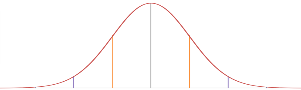
This graph provides another way to think about the distribution of the data.
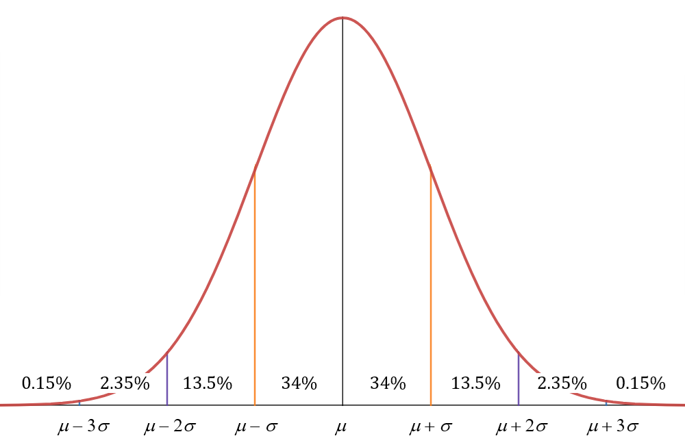
Because [latex]68\%[/latex] of the data are within one standard deviation of the mean, we have [latex]34\%[/latex] of the data slightly below the mean and [latex]34\%[/latex] slightly above. Moving outwards one more standard deviation in each direction, we have another [latex]13.5\%[/latex] below the mean and another [latex]13.5\%[/latex] above the mean, encompassing a total of [latex]95\%[/latex] of the data. Moving outwards one more standard deviation, we have another [latex]2.35\%[/latex] far below the mean and another [latex]2.35\%[/latex] far above the mean, bringing the total up to [latex]99.7\%[/latex] of the data. This leaves only [latex]0.15\%[/latex] of the data more than three standard deviations below the mean and [latex]0.15\%[/latex] of the data more than three standard deviations above the mean.
Practice Exercises
Around [latex]16\%[/latex] of U.S. males in their forties weigh less than [latex]160[/latex] lb and [latex]16\%[/latex] weigh more than [latex]230[/latex] lb. Assume a normal distribution.[3]
- What percent of U.S. males weigh between [latex]160[/latex] lb and [latex]230[/latex] lb?
- What is the average weight? (Hint: think about symmetry.)
- What is the standard deviation? (Hint: You have to work backwards to figure this out, but the math isn't complicated.)
- Based on the empirical rule, about [latex]95\%[/latex] of the men should weigh between _______ and _______ pounds.
This version of the graph can help us group the data into general categories. This is not official terminology, but hopefully it gets the point across.
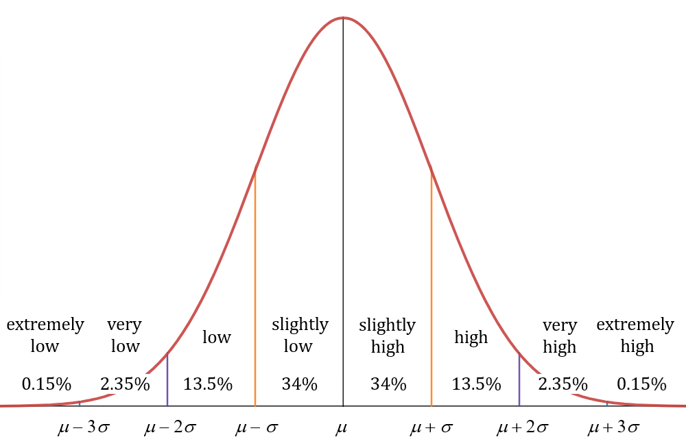
Looking at the middle [latex]68\%[/latex] of the data, [latex]34\%[/latex] could be considered "slightly low" and [latex]34\%[/latex] could be considered "slightly high". Moving outwards, we have another [latex]13.5\%[/latex] that could be considered "low" and another [latex]13.5\%[/latex] could be considered "high". Moving outwards again, we have another [latex]2.35\%[/latex] that could be considered "very low" and another [latex]2.35\%[/latex] that could be considered "very high". Finally, [latex]0.15\%[/latex] of the data could be considered "extremely low" and [latex]0.15\%[/latex] could be considered "extremely high".
We can find the standard deviation of a data set using the formula below. To summarize the formula, the standard deviation is the square root of the average difference of each number in the data set from the mean of that data set. Let's take a look at how that is calculated in the examples below.

 |
= | population standard deviation |
 |
= | the size of the population |
 |
= | each value from the population |
 |
= | the population mean |
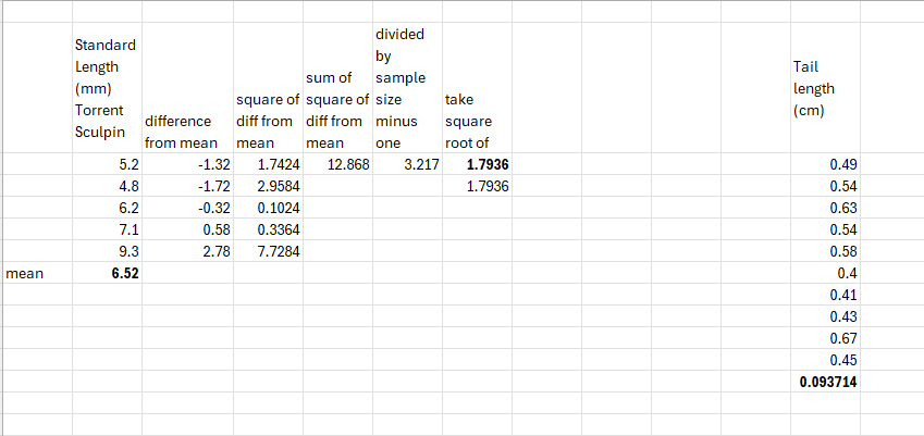
Examples: Calculating the standard deviation
A) Find the standard deviation by hand.
| Standard Length (cm) Torrent Sculpin
5.2 |
|
| 4.8 | |
| 6.2 | |
| 7.1 | |
| 9.3 | |
B) Use Excel to perform the standard deviation calculations.
| Tail length (cm) |
| 0.49 |
| 0.54 |
| 0.63 |
| 0.54 |
| 0.58 |
| 0.40 |
| 0.41 |
| 0.43 |
| 0.67 |
| 0.45 |
If you are asked only one question about the empirical rule instead of three in a row ([latex]68\%[/latex], [latex]95\%[/latex], [latex]99.7\%[/latex]), you will most likely be asked about the [latex]95\%[/latex]. This is related to the "[latex]95\%[/latex] confidence interval" that is often mentioned in relation to statistics. For example, the margin of error for a poll is usually close to two standard deviations.[4]
Let's finish up by comparing the performance of three NFL teams at the beginning of this century.
Practice Exercises
The numbers of regular-season games won by the New England Patriots[5] each NFL season from 2001-2019: [latex]11[/latex], [latex]9[/latex], [latex]14[/latex], [latex]14[/latex], [latex]10[/latex], [latex]12[/latex], [latex]16[/latex], [latex]11[/latex], [latex]10[/latex], [latex]14[/latex], [latex]13[/latex], [latex]12[/latex], [latex]12[/latex], [latex]12[/latex], [latex]12[/latex], [latex]14[/latex], [latex]13[/latex], [latex]11[/latex], [latex]12[/latex].
The mean number of wins is [latex]12.2[/latex], and a spreadsheet tells us that the standard deviation is [latex]1.7[/latex] wins.
- There is a [latex]95\%[/latex] chance of the Patriots winning between _______ and _______ games in a season.
- In 2020, the Patriots won [latex]7[/latex] games. Could you have predicted that based on the data? How many standard deviations from the mean is this number of wins?
The numbers of regular-season games won by the Buffalo Bills[6] each NFL season from 2001-2019: [latex]3[/latex], [latex]8[/latex], [latex]6[/latex], [latex]9[/latex], [latex]5[/latex], [latex]7[/latex], [latex]7[/latex], [latex]7[/latex], [latex]6[/latex], [latex]4[/latex], [latex]6[/latex], [latex]6[/latex], [latex]6[/latex], [latex]9[/latex], [latex]8[/latex], [latex]7[/latex], [latex]9[/latex], [latex]6[/latex], [latex]10[/latex].
The mean number of wins is [latex]6.8[latex], and a spreadsheet tells us that the standard deviation is [latex]1.7[/latex] wins.
- There is a [latex]95\%[/latex] chance of the Bills winning between _______ and _______ games in a season.
- In 2020, the Bills won [latex]13[/latex] games. Could you have predicted that based on the data? How many standard deviations from the mean is this number of wins?
The numbers of regular-season games won by the Denver Broncos[7] each NFL season from 2001-2019: [latex]8[/latex], [latex]9[/latex], [latex]10[/latex], [latex]10[/latex], [latex]13[/latex], [latex]9[/latex], [latex]7[/latex], [latex]8[/latex], [latex]8[/latex], [latex]4[/latex], [latex]8[/latex], [latex]13[/latex], [latex]13[/latex], [latex]12[/latex], [latex]12[/latex], [latex]9[/latex], [latex]5[/latex], [latex]6[/latex], [latex]7[/latex].
The mean number of wins is [latex]9.1[latex], and a spreadsheet tells us that the standard deviation is [latex]2.6[/latex] wins.
- There is a [latex]95\%[/latex] chance of the Broncos winning between _______ and _______ games in a season.
- In 2020, the Broncos won [latex]5[/latex] games. Could you have predicted that based on the data? How many standard deviations from the mean is this number of wins?
Problem Set 9.2
1) Find the standard deviation.
| Length of 4th metatarsal (mm) |
| 10.2 |
| 12.4 |
| 11.1 |
| 10.5 |
2) Which data set has more variation?
| Selway (g) | North Fork (g) |
| 15 | 12 |
| 13 | 13 |
| 14 | 11 |
| 18 | 13 |
| 22 | 15 |
| 17 | 11 |
| 14 | 13 |
| 12 | 32 |
3) Think like a forester. Here are age data from plots in three different stands. Which stand likely grew on a site that was clear cut? How do you know? Use standard deviation to support your answer.
| Stand 1
79 |
Stand 2 | Stand 3
148 |
||
| 80 | 90 | 92 | ||
| 78 | 76 | 158 | ||
| 82 | 82 | 111 | ||
| 81 | 76 | 136 | ||
| 83 | 68 | 195 | ||
| 80 | 67 | 6 | ||
| 81 | 74 | 17 | ||
| 83 | 79 | 80 | ||
| 77 | 65 | 205 | ||
| 80 | 83 | 186 | ||
| 81 | 79 | 140 | ||
| 75 | 111 | 3 | ||
| 80 | 100 | 108 | ||
| 81 | 69 | 74 | ||
| 77 | 86 | 206 | ||
| 82 | 80 | 113 | ||
| 79 | 64 | 5 | ||
| 80 | 44 | 5 | ||
| 81 | 88 | 78 | ||
| 82 | 82 | 82 | ||
| 80 | 84 | 173 | ||
| 80 | 81 | 11 | ||
| 82 | 75 | 48 | ||
| 77 | 78 | 109 |
- Well, there is a formula, [latex]y=\frac{1}{\sqrt{2\pi}}e^{-\frac{x^2}{2}[/latex], but it was discovered after the fact. ↵
- I eyeballed it and it seemed like a reasonable assumption. ↵
- Source (PDF file): https://www2.census.gov/library/publications/2010/compendia/statab/130ed/tables/11s0205.pdf ↵
- Source: https://en.wikipedia.org/wiki/Standard_deviation ↵
- Source: https://www.pro-football-reference.com/teams/nwe/index.htm ↵
- Source: https://www.pro-football-reference.com/teams/buf/index.htm ↵
- Source: https://www.pro-football-reference.com/teams/den/index.htm ↵
