Chapter 13: Formulas – Operations

What We’ll Cover >>>

• Formula Basics
• Parts of a Formula
• Basic Formulas
• Auditing Formulas
• Quick Analysis Tool
• Common Error Codes

This section reviews the fundamental skills for entering formulas into an Excel worksheet. Excel is used for many kinds of calculations: mathematical, statistical, financial, scientific, reference lookups, and more. It is useful in many types of business, and is a key tool in cleaning, calculating, and analyzing data.

Formula Basics

A main strength of Excel is that you can use it to calculate data in many ways. Calculations allow for the development of additional data for analysis and decision making. A spreadsheet full of employees, their salaries, and the value of their benefits packages is useful. Calculating the annual and quarterly costs can be more useful in using for comparisons, preparing for taxes, etc.

Excel formulas are an expression that operates on values in a range of cells and return a result. They let you do calculations like addition, subtraction, multiplication, and division.

Excel functions are also formulas, but they are predefined by Excel for particular business purposes and perform calculations by using specific values, called arguments, in a particular order, or structure.

Formula bar

We’ve used the formula bar a bit when not directly inputting data into Excel cells. The formula bar reflects what is in a cell. However, its power comes from the ability to write and process formulas, to display named ranges and how the formula is organized, and in helping identify errors.

In the example, the formula bar is displaying a simple calculation for Cell A1. To the left of the field, the small fx icon is a way to open the Functions panel and access to the Excel functions library. The checkmark (green when it is active) is a way to approve a formula instead of simply pressing Enter. The X icon (red when it is active) is important because it allows you to back out of the formula bar without saving what is in it. Why is that useful? It can be all too easy to accidentally click in the wrong cell and corrupt a working formula, and the red X lets you stop before you can save and exact the corruption, error, etc.

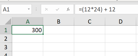
MedAttrib: author-generated. MS Excel formula bar.

Formula Ribbon

In Excel, you can manually input formulas, as we did in the earlier chapter on click-linking to data cells. You can also use the Excel Formula tab/ribbon to access common predefined functions and to look up a wide variety of pre-built formulas in the Excel function library. This is also where we have found the Name Manager tools for naming ranges in a dataset. Those named ranges show up in formulas in a way that keeps a formula from seeming to access random and long strings of cell range information. The named ranges add context in a formula, especially for troubleshooting.

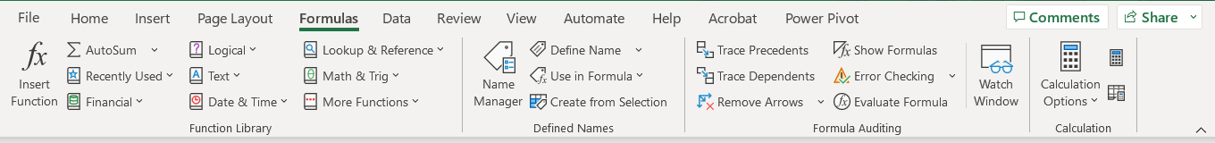
MedAttrib: author-generated. MS Excel Formula ribbon.

The Excel Function Library

Users can access the Function Library from the Formulas tab by clicking on the Insert Function icon. The Insert Function panel opens and allows for a search of formula-related keywords. You can also try to browse through the category dropdown. This is useful to people who work in specific industries in which they use a lot of calculations and know just what to look for, whereas for basic workplace talent, most of the available functions won’t mean anything or be useful. The use is in context of one’s training in specific career areas requiring calculations.

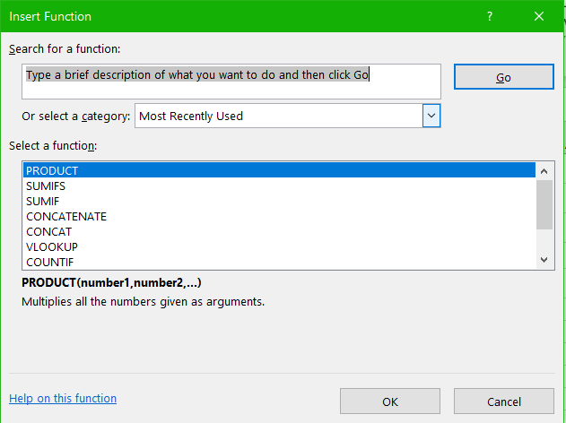
MedAttrib: author-generated. MS Excel Insert function / Function Library access.

TIP: Faster Function library access. Click the FX symbol to the left of the Formula Bar, which opens the Insert Function dialog box. Or you can press SHIFT F3 (function button).

Thinking out formula scenarios

A key part of succeeding in using any formula or function is to know exactly what you want to accomplish. Students in numbers and data-heavy fields are usually learning the skills for what calculation processes are needed for their field (scientific, accounting, higher-level math, research, etc.), and Excel is a tool to accomplish that. Students in fields that don’t work with a lot of data or computations can have trouble formulating the scenario, or words, for what needs to be calculated and why/how. Yet, we need to be able to do this to decide what formula to write or find in the Functions.

Steps

First, keep in mind that any calculation is a kind of combination of a story problem (UGH!) and a test of logic.

• How much is a “service”?
• What is a bonus for a high achieving real estate agent?
• How many products were sold in the last 3 months?
• How many days are in a class quarter?
• If you know someone’s name and look it up in a table, can you tell what region they represent or how much property they sold or what grade they earned?

SO, the first thing you have to do is make sure you understand exactly what is being asked. Then you need to figure out what exactly you are trying to reference – to look at – so you can pull out the information you need. Then you need to ask Excel the right kind of question in terms Excel can calculate from.

Here’s something I learned when I first took a class in basic programming:

• Write out what I think that I’m being asked to do.
• Drink coffee (or fave beverage).
• Write out what steps I think I would need to do to get at the information.
• More coffee.
• Look up / research Excel information to see what the types of calculations I need to do might require.
• Think about stronger coffee, but likely go for calming tea or water.
• Study the basic logic and format of a calculation to see if it can do what I need.
• Take a break for a serious treat or rest.
• Experiment.

Say you are being asked to get a total of the sales from the 8 sales reps who sell coffee to 3 cafes. You would figure (rightly) that you need to see a list of all their sales, then get a total of those numbers. You would be looking to get a grand totals response in terms of currency.

Say you need to find out which coffee roasts sold well over Fall 2022? You would need to figure out how to ask Excel to look up the column of roast flavors, see the quantities sold, and look at this info for only the months of September, October, November, and December 2022. You would need more information to find out if you are supposed to find the count for each coffee, or the dollar amount sold, etc. Then you would need a way to either do a subtotal table, or a lookup table, etc.

Say you (as a teacher) have 30 students who have finished the class and need you to calculate their final grades. You need to know the students’ names, their final points, and some table of what points are equal to what publishable numeric grade. You would need to do some kind of lookup and have the response calculate into your student roster next to their point count so you could accurately update the school grades with the right numeric grade (4.0, 3.8, etc.)

You usually have to logically process what is being asked, and carefully decide what is needed. Take your time, map it out if you need to, and even write a layman’s English (or your own first) Language process. Then figure out how to ask Excel to calculate it for you. The Excel Functions menu tab/ribbon and Functions lookup provides wizard windows for every function, so if you know what I need to look for, you can use those quite handily.

Parts of a Formula

When you make a formula in Excel, there are several different components that supply the source data to the formula and express what operations should be performed on that information. Depending on the formula type, you may need include any or all of the following items:

• Starting the formula: In order for Excel to know the cell content will be a formula to be calculated, you need to start by typing the EQUAL sign = This tells Excel that the contents of the cell will be an answer to a question (equal to), rather than a string of text or a basic numbers to format in some way.

Your mandatory BFF for all formulas – the EQUAL sign.

• Constants: Numbers or text values that you enter directly in a formula, like =2*3. This is a manual way of telling a formula what to calculate with.
• Cell reference: A reference to a cell that contains the value (item) you want to use in your Excel formula, e.g. =SUM(A1, B2, C3). This allows you to create formulas that can be copied and reused, rather than requiring a manual input of the numbers yourself.
• Range reference: To refer to data in two or more contiguous cells, you use a range reference like A1:A5. For example, to sum values in all cells between A1 and A8, inclusive, use this formula: =SUM(A1:A8)
• Named range reference: A defined name for a cell range, constant, table, or function, such as =SUM(TaxCol). In earlier chapters we created and used named data ranges in part to prepare for working with formulas.

Operators

Operators: These are special symbols that specify the type of operation or calculation to be performed, such as +, *, etc. They tell Excel what the operation, or calculation method, is to be, like sum, quotient, division, etc. For this chapter, we’ll only look at arithmetic.

• Addition: + (plus sign)
• Subtraction: – (minus sign)
• Multiplication: * (asterisk)
• Division : / (forward slash)
• Percent: % (percent sign)
• Exponentiation: ^ (caret)
• Equal to: =
• Greater than: > (greater than sign)
• Less than: < (less than sign)
• Greater than or equal to: >= (greater than or equal to sign)
• Less than or equal to: <= (less than or equal to sign)
• Not equal to: <> (not equal to sign)

The order in which calculation is performed can affect the return value of the formula, so it’s important to understand the order, and to use parentheses to change the order to obtain the results you expect to see. If a formula contains operators with the same precedence — for example, if a formula contains both an addition and subtraction operator — Excel evaluates the operators from left to right. Otherwise, you will want to use parentheses to separate/clarify sections of a formula. For instance, multiplication and division happen before addition and subtraction.

=12+5*3  would be 27

=(12+5)*3 would be 51

Excel uses the standard mathematical order of operations. When writing complex formulas it is important to remember this order of operations. You want to be sure that your formulas will calculate in the order you intend. To help you remember which operations will be performed first, you can use the acronym PEMDAS.

P – parentheses

E – exponents

MD – multiplication and division

AS – addition and subtraction

Cell References

Cell References are a way to refer to the contents of a cell.

• Absolute: Absolute references remain constant, no matter where they are copied.
• Relative: Relative references change when a formula is copied to another cell. This allows a formula to be reused and to pick up the contents of the record around it so that you don’t have to manually input all numbers (constants) yourself.
• Selection: You select one or more cells while creating a formula or a location reference in another table and/or worksheet.
• Named: You can Define a Name of a cell so that the cells remain stable in a formula that you copy and paste for further use in other cells in a column. This would be an Absolute reference. Otherwise, the pasted formula will change the cell’s location reference to be relative to the new row it is seeking to create the formula for. Example: =Fee*20, where the cell I5 has been named FEE, is more stable than =I5*20. Other formulas needing the contents of cell I5 would use the named reference FEE instead.
• Circular Reference: This happens when a formula is trying to calculate itself, and you have an Excel feature called iterative calculation turned off. It can also happen during indirect references in a formula. It results in errors.

Note: Formulas can be written with only relative references, with only absolute references, or with mixed references.

Basic Formulas

In this chapter, we will keep things straightforward and will work with basic mathematical formulas.

ACTION: Try Me activity

We will work with the Taste du Monde workbook, named Ch13–Calculations.xlsx. Make a copy of the file for your Examples folder, then open that copy.

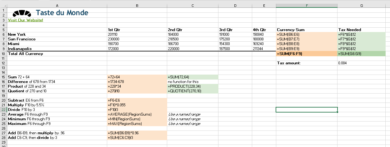
Here is what we are aiming for:

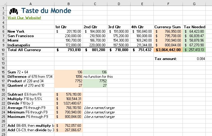
MedAttrib: author-generated. MS Excel Ch14 finished calculations.

The workbook has only one sheet, which is more of a worksheet than a practical company ledger.

Let’s start with the basic manual math.

The formulas begin with the = sign, to tell Excel something is being calculated, an answer will be provided.

Remember: Your mandatory BFF for all formulas – the EQUAL sign.

• Cell B15 needs to add 72 and 64, which is a sum. In B15, type =72+64 with no spaces.
• Cell C15 can use this function instead: =SUM(72, 64)
• Cell B16 needs to subtract 678 from 1734, which is a difference. = 1734-678. 
  • NOTE: There seems to be no comparable subtraction function in Excel.
• Cell B17 needs to multiply 228 and 34, which is a product. =228*34
• Cell C17 can use this function instead: =PRODUCT(228, 34)
• Cell B18 needs to divide 279 by 10, which is a quotient. =270/10
• Cell C18 can use this function instead: =QUOTIENT(270, 10)
• SAVE your work.

Relative References

Relative: Relative references change when a formula is copied to another cell.  What this means is that if you create a formula to sum up the total numbers of a row, then paste that same formula down one cell to sum up the total numbers of the next row, Excel will assume you want the references to the cells with the numbers in the new row to change inside the pasted formula.

Row 1’s Cell D1: cell A1 + cell B1 + cell C1 would equal the total of the numbers in those 3 cells. The formula in cell D1 would be =A1+B1+C1

Then, pasting  =A1+B1+C1 into Row 2’s cell D2 would automatically change it to =A2+B2+C2, because Excel assumes you want the formula to calculate the proper total for Row 2 information. This is what a “relative” reference in a formula in Excel means.

Relative references in a formula allow a formula to be reused and to pick up the contents of the record around it so that you don’t have to manually input all numbers (constants) yourself.

Now, let’s add some of the things in the Taste du Monde table.

• Cell F6 needs to add cells B6-E6, and because there are several numbers, the Excel formula that uses a Relative reference to those cells will do the job: =SUM(B6:E6)
• Cell F7 needs to add cells B7-E7. Let’s copy the formula from cell F6 and paste it into cell F7 and learn what happens.

NOTE: Relative Reference. Copying the formula from Cell F6 and pasting it Into Cell F7, and having that change the formula to calculate the sum of Cells B7-E7, is an example of Relative References. Excel was able to adjust the formula to be relative to the data related to Cell F7, instead of simply copying the exact numbers from Cells B6-E6.

• Cell F8 needs to add cells B8-E8. Copy the formula from cell F6 and paste it into cell F8.
• cell F9 needs to add cells B9-E9. Copy the formula from cell F6 and paste it into cell F9.
• Now, we cannot do this for cell F10. Why? Because cell F10 is supposed to be the sum of Cells F6-F9, the cells above it in the column.
• Type =SUM(F6:F9)

Let’s get a little more experience and range. Rows 17-22 ask for a little more, and we’ll need to think about the order of operators – the order of what we calculate – when more than one calculation is happening in the formula.

• Cell B20: =F6-E6
• Cell B21: =F10*0.055
• Cell B22: =F10/3
• SAVE your work.

Before we calculate the next three, it would be useful to create a named data range instead of referring to the range of cells more manually.

• Select Cells F6 through F9, then use the Formulas tab, Defined Names group, Define Name dropdown, Define Name selection, and type RegionSums in the Name field, then click OK.

Now these three functions should work properly as typed:

• Cell B23: =AVERAGE(RegionSums)
• Cell B24: =MIN(RegionSums)
• Cell B25: =MAX(RegionSums)
• Then, lets also try B27: =SUM(B6:B9)*0.96
• B28: =SUM(C6:C9)/3
• SAVE your work.

Absolute References

Absolute references remain constant, no matter where they are copied. This means that the number inside a specific cell (like a tax rate or a specific discount percentage) should remain the exact same info in every instance of a formula it is used in. This is useful if you need one value (number) in a formula to remain the same no matter what rows of data are being calculated against it. We’ll do this with the Tax Needed cells in column G.

An absolute reference is referred to differently in a formula / function. The idea is the tell Excel to freeze the reference so that it remains static – the same cell, no matter how it is used in a column that might otherwise auto-calculate relative references for you.

The Absolute reference format uses a dollar symbol ($) before the cell’s coordinates to make the cell reference fixed/absolute. An example would be referring to the Cell G12 – a tax amount – as $G$12 in a calculation. Let’s try.

• Cell G6: =F6*$G$12    This is to calculate the tax needed for the New York currency sum.
• Cell G7: Copy cell G6 and paste in cell G7. Notice the formula still refers to the tax info in $G$12, which is absolute to Cell G12, which is what we want. Yet, the relative reference to cell F6 changes to F7 to let Excel calculate the tax needed relative to the San Fransisco currency sum.
• Cell G8: Copy cell G6 and paste in cell G8.
• Cell G9: Copy cell G6 and paste in cell G9.

Again, we cannot do this for cell G10. Why? Because cell G10 is supposed to be the sum of cells G6-G9, the cells above it in the column.

• Type =SUM(G6:G9)
• SAVE your work.

TIP: Use Universal Constants. There will be times when you are writing formulas that you will need to use universal constants, or numbers that do not change, such as the number of days in a week, weeks or months in a year, and so on. For example, if you are calculating the monthly cost of an item when you know the yearly cost, you will always divide by 12 since there are 12 months in a year. In this case, you use the constant of 12 instead of a cell reference because the number of months in a year never changes.

Auditing Formulas

Excel provides a few tools that you can use to review the formulas entered into a worksheet. For example, instead of showing the outputs for the formulas used in a worksheet, you can have Excel show the formula as it was entered in the cell locations. This is demonstrated as follows:

• With the Ch13Calculations.xlsx file open, click the Formulas tab of the ribbon.
• Click the Show Formulas button in the Formula Auditing group of commands. This displays the formulas in the worksheet instead of showing the mathematical outputs.

MedAttrib: author-generated. MS Excel Ch13 finished calculations showing formulas.

• Click the Show Formulas button again. The worksheet returns to showing the output of the formulas.

You can also toggle Show Formulas on and off using the keyboard. Hold down the CTRL key while pressing the ` key.

Keyboard Shortcut: Show Formulas. Hold down the CTRL key while pressing the accent symbol.

Two other tools in the Formula Auditing group of commands are the Trace Precedents and Trace Dependents commands. These commands are used to trace the cell references used in a formula. A precedent cell is a cell whose value is used in other cells. The Trace Precedents command shows an arrow to indicate the cells or ranges (precedents) which affect the active cell’s value. A dependent cell is a cell whose value depends on the values of other cells in the workbook. The Trace Dependents command shows where any given cell is referenced in a formula. The following is a demonstration of these commands:

• Click cell G12.
• Click the Trace Dependents button in the Formula Auditing group of commands in the Formulas tab of the ribbon. A blue arrow appears, pointing to cell G6. This indicates that cell D3 is referenced in a formula entered in cell F3.
• IF NEEDED for an instructor’s assignment, SCREENSHOT HERE.
• Click the Remove Arrows command in the Formula Auditing group of commands in the Formulas tab of the ribbon.

This removes the Trace Dependents arrow.

• Click cell F10.
• Click the Trace Precedents button in the Formula Auditing group of commands in the Formulas tab of the ribbon. A blue arrow with dots in cell F6, and pointing to cell F10 appears. This indicates that cells D3 and E3 are references in a formula entered in cell F3.
• Click the Remove Arrows command in the Formula Auditing group of commands in the Formulas tab of the ribbon.

This removes the Trace Precedents arrow.

• SAVE your work.

Quick Analysis Tool

The Quick Analysis Tool allows you to create standard calculations, formatting, and charts very quickly.

• Mac Users: the Quick Analysis Tool is not available with Excel for Mac. There are alternate steps for Mac Users below.

Be sure to press CTRL ~ to return your spreadsheet to the normal view (the formula results should display, not the formulas themselves).

• Select the range of cells B6:E9.
• In the lower right corner of your selection, you will see the Quick Analysis tool (see Figure 3.4).

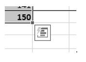
MedAttrib: author-generated. MS Excel Quick Analysis pop-up.

When you click on it, you will see that there are a number of different options. This time we will be using the Totals option.

• Select Totals, and then the SUM option. Selecting that SUM option places =SUM() calculations in row 10.
• SAVE your work and close the file. We’re done with it.

Common Error Codes

Excel presents a number of error codes when a formula doesn’t work properly. And, for learners who work with Excel for standard/casual practice, the codes may not mean a lot or tell you exactly how to fix the problem. Excel tends to be somewhat obtuse in explaining a problem, because the explanation is general to the “type” of issue the program can’t resolve, not the exact nature of your actual formula and formula data. SUPER ugh!

However, when you get one of these, Excel does offer you a small green or yellow icon right by the error formula that you can click for a link to some help. There also tend to be Microsoft error code info pages, and responses to doing an Internet search.

These codes should give you something to start with,

• #DIV/0! Trying to divide by 0
• #N/A! A formula or a function inside a formula cannot find the referenced data
• #NAME? Text in the formula is not recognized
• #NULL! A space was used in formulas that reference multiple ranges; a comma separates range references
• #NUM! A formula has invalid numeric data for the type of operation
• #REF! A reference is invalid
• #VALUE! The wrong type of operand or function argument is used