Chapter 14: Functions – Data Management
What We’ll Cover >>>
- Concatenation
- Proper Punction
- Text to Columns
- Left/Right Functions
- Hyperlink Function
A lot of data you will use in Excel may be text, as well as numbers. You may inherit spreadsheets with data in inconsistent formats, such as when it is imported from other sources or added manually from data entry. You may be tasked with making existing data which works very well in the workbook appear differently to be better able to be viewed in charts and output materials. Various functions exist that allow you to do these things, without actually being functions that calculate number. These functions are for Data cleanup. Here are a few common ones:
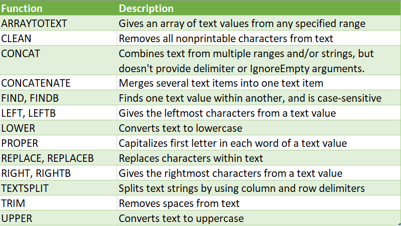
MedAttrib: author-generated. MS Excel data management functions.
In this chapter, we’ll practice four common ones so that you can get a feel for what you can accomplish.
Proper Function
ACTION: Try Me activity
We will work with a Prisvard Tech workbook, named Ch14-Concat.xlsx. Before you start working, go to your DataFiles folder and make a copy of the file for your Examples folder, then open that copy. Let’s see what we are aiming for:
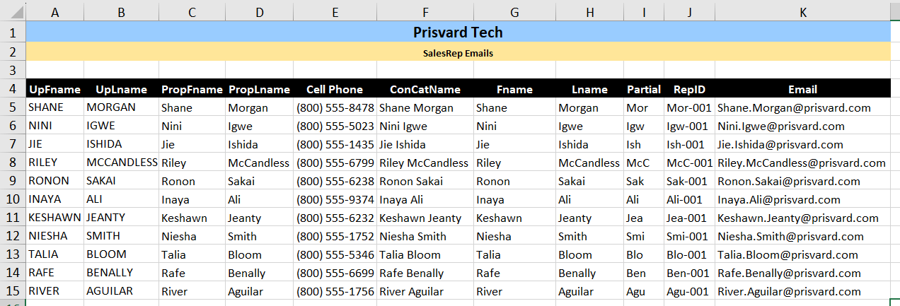
MedAttrib: author-generated. MS Excel Data Management results.
The workbook has only one sheet, named SalesReps. It is mostly empty, and needs us to create new email addresses for the reps. The names are currently in uppercase, and in two columns, which will be hard to make email addresses from.
We’ll work from left to right to accomplish several data conversion tasks until we can create the email address for each rep.
Like numeric/calculation formulas and functions, these formulas begin with the = sign, to tell Excel that something is being changed and that an answer will be provided.
- Click on cell C5. We need to convert cell A5 from allcaps to a proper format, from SHANE to Shane. We will do this in cell C5 which is the column called PropFName.
- We’ll use the Proper function, which changes the case of letters in text data for us. We’ll need to find the function.
- While in cell C5, click the FX insert function symbol just to the left of the Formula bar.
A dialog box opens:
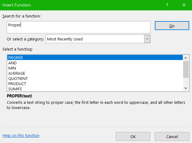
MedAttrib: author-generated. MS Excel data Insert Function dialog box.
- In the “Search for a function” field, type Proper, then click GO.
- From the list of resulting functions, choose Proper, then click OK.
Another dialog box will open: Function arguments.
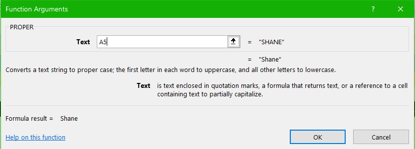
MedAttrib: author-generated. MS Excel data Function Arguments dialog box.
This dialog box asks you to tell you want should be converted. The easiest way is to either type the name of the cell to be converted, or to click on the cell.
TIP: Cell referencing in Function dialog fields. While building a function/formula, including while in a Function dialog box, you can click on a cell in your worksheet to reference it in a cell. Leave the dialog box open, find the cell in your workbook, click on it, and the reference will appear in the dialog box field.
- While in the dialog box, click on cell A5. The dialog box will populate the field with the contents of A5 (SHANE), preview what it looks like, and preview what the results of the function will be (Shane).
- Click OK to finish the function calculation.
We need to do the same thing to Shane’s last name in cell D5.
- Click on cell D5, and click the FX insert function symbol just to the left of the Formula bar. The Insert Function dialog box will open, and the first item in the list will likely be PROPER since we just used it. Click that top open the Function Arguments box.
- In the dialog’s Text field, type B5, and review the previews before clicking OK.
- Let’s copy this function through the remaining C and D column.
- Select cell C5 and D5, CTRL C to copy (CMD C for Mac), then paste them into cells C6-D15. This will populate the proper first and last names for us.
Cell D8 has a problem, which we will have to handle manually. Mccandless should be McCandless per conventional spelling of a name beginning “Mc”.
- Select cell D8, copy it, and use Paste Values to replace the formula with the text results of the formula. This way, you can change the cell contents manually without interfering with a formula.
- In cell D8, change Mccandless to McCandless.
Concatenation
Next, we need to merge the contents of the C column cells and D column cells together so that we can have both the first and last name of the Sales Reps in the same column. This will allow us to use them to build and email address. We will use the Concatenate function, which lets us set up a formula that also accounts for adding space between the first and last names.
- Click in cell F5, and use the FX symbol by the formula bar to open the Insert Function Dialog.
- In the search field, type concate, and click GO.
- Choose Concatenate, which opens the Function Arguments dialog.
In this case, the function starts with 2 fields, since the function is about combining more than one cell/piece of data. I our case, we will need 3 (three). Pay attention below.
- In the first field, type C5.
In the second field, we actually have to specify that we need a space between the first and last name in the function results, or the first and lastname will appear as ShaneMorgan. We also have to use quote marks to reference the space, because Excel expects that all arguments in a function are the data contents of a cell, not something you insert from another source.
- In the second field, type “ “ which is an open quote, a space, and a closed quote.
Note that a third field appears as you use the second field. Excel can string together several items to make a concatenation, and adds fields as you use one so that you have the option to populate them with needed data.
- In the third field, type D5, then click OK.
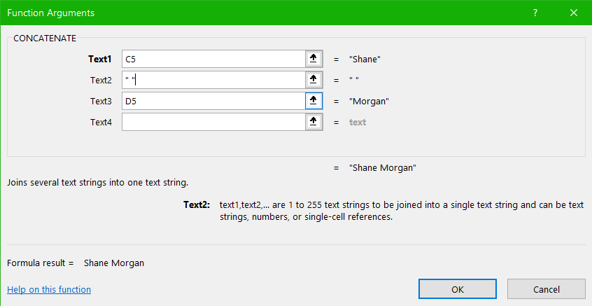
MedAttrib: author-generated. MS Excel data Function Arguments for Proper dialog box.
Cell F5 now should show Shane Morgan, which is the joining of the contents of cells C5 and D5.
- Copy the contents of Cell F5 into cells F6-F15 to populate them with the data.
- SAVE your work.
Text to Columns
This is a good time to find out how to separate data in one column into two columns. For this to work, however, Excel needs the data to be separated to be a static value, not the results of a formula.
- Select cells F5-F15, copy, and paste the range over itself as Paste Values. This removes the formula while retaining the results of the formula.
Next, let’s separate the contents of cell F5 into cells G5 and H5.
- Select cell F5, the go to the Data ribbon, Data Tools group, and click the Text to Columns icon.
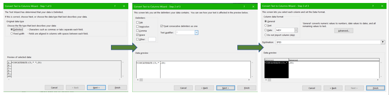
A Wizard will open. We need to tell this wizard that Shane Morgan (2 words with a space between them) needs to be separated into one word for each of Cell G5 and H5.
TIP: Excel Wizards. Excel has a few Wizard mini apps that are like built-in action macros, They have several steps that allow you to make choices so that Excel can perform an otherwise complex action for you.
In the Wizard, you are in Step 1, which asks for you to interpret the original data type. Ours is delimited, because the text has been delimited (positioned) by a space.
- Click Next.
- Choose the Delimiter (item that affected the placement of Shane and Morgan, which is the space between them). You may have to uncheck every one, then choose only the Space delimiter.
- Click Next.
The third step needs you to tell Excel where the new data will go. Because the data will be split into 2 columns (first and last name), it will need 2 empty columns already available to put the split into. We have them, with columns G and H. However, Excel needs you to only specify the first of the columns and it will populate both columns for us.
- In the Destination field, type $G$5 to specify a fixed place. An Absolute reference is needed so only that one cell is referred to.
- Click Finish.
- SAVE your work.
MedAttrib: author-generated. MS Excel Text to Columns wizard.
Observe that cell G5 should have Shane in it, and H5 should have Morgan in it.
There is one problem. The contents of cells G5 and H5 are not actually formulas for you to copy and paste down. The column split worked for only one row.
Let’s do the rest.
- Select cells F6-F15.
- Click the Data ribbon’s Text to Columns icon.
- In Step 1, make sure that Delimited is selected, then click Next.
- In Step 2, make sure that only Space is check marked, then click Next.
- In Step 3, in the Destination, type $G$6, then click Finish.
Cells G6-H15 should now be populated.
- Because they default populated in a centered text alignment, use the Home tab Format Painter to select the Format of cell D5 and apply it to Cells G5-H15.
- SAVE your work.
LEFT/RIGHT Functions
Next, we want to capture only part of a Sales Rep’s name for a new creation of a RepID. We’ll use column I for the formula for this, and use the LEFT function to capture the first 3 letters of the SalesReps last names.
- Select Cell I5.
- Click the FX symbol by the Formula bar, and in the search, type left.
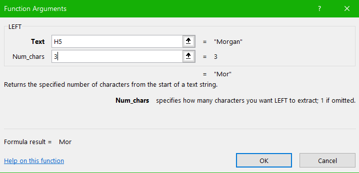
- Double-click the LEFT entry in the resulting list.
- In the Function Arguments dialog, type the needed Cell you plan to get the letters from, which is H5.
- In the Num_Chars field, type 3, so that we can get the first 3 letters of the last name.
- Click OK.
- SAVE your work.
MedAttrib: author-generated. MS Excel LEFT Function Arguments dialog.
- In Cell I5, you should see Mor. It is centered text, so left align it.
- Copy Cell I5 into I6-I15. This should populate the working formula down the rest of the data range’s column.
Let’s concatenate the Column I partial names with a number to make a SalesRep ID number in column J.
- Click cell J5, and then click the FX symbol by the formula bar (or choose Formulas ribbon, Insert Function icon).
- In the search field, type concat, and click GO.
- Choose Concatenate from the list and click OK.
- In the Function Arguments, type I5 in the first text field.
- In the second field, type “-“ (quote dash quote).
- In the third field, type “001”
- Click OK. You should now see Mor-001 in cell J5.
- Left-align cell J5.
- Copy cell J5 to J6-J15. This will populate these cells with the relative SalesRep ID numbers.
Finally, let’s create the email address. This will also be a concatenation of several fields this time.
- Click cell K5, and then click the FX symbol by the formula bar.
- Choose Concatenate from the list and click OK.
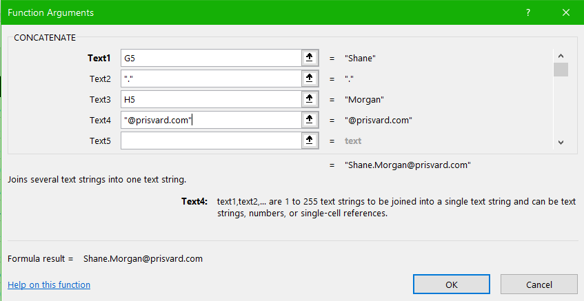
- In the Function Arguments, type G5 in the first text field.
- In the second field, type “.“ (quote period quote).
- In the third field, type H5
- In the fourth field, type “@prisvard.com” with the quote marks.
- Click OK. This should give you Shane.Morgan@prisvard.com in cell K5.
- Left-align cell K5.
- Copy Cell K5 to K6-K15. tot populate these cells with their relative email addresses.
MedAttrib: author-generated. MS Excel CONCATENATE Function Arguments dialog.
- SAVE your work, and close the file. We’re done!
Hyperlink Function
Hyperlinks are active links to different locations, like to a website, to an email address, and to another location in a existing file. We see them frequently in websites – their navigation links, their link to their comment and sign-up forms, their links to other websites and online resources, etc. Hyperlinks can be and are used in documents off the web, too. For instance, in a master’s thesis or a novel written in a Word document, the table of contents will link to ‘anchors’ in the paper’s pages that begin sections or chapters. In Excel, hyperlinks are useful to link to external websites, as an example.
Excel has multiple ways of adding/editing hyperlinks. You can set Excel to default to automatically changing a text URL (website or email address) to an active clickable link. You can manually add hyperlinks as you need them. Or, you can use a function that will allow you to add or edit multiple hyperlinks at one time.
Default Hyperlinks
In Excel, you can set the program to automatically change the text for a website URL or online email address to a clickable hyperlink. Actually, this is already the default, but sometimes you might want to turn it off. Why?
When an Excel cell has an active hyperlink in it, the whole cell act like the clickable hyperlink. When you select the cell to edit it, the hyperlink will click and try to pen your computer’s default browser then go to the hyperlinked URL. This can get annoying.
In Excel’s backstage area – accessed on the PC through the File tab, you can find the hyperlink setting under Options / Proofing / Autocorrect Options, and in the resulting Autocorrect dialog window, under the Autoformat as you type tab. The actual command is “Internet and network paths with hyperlinks “, and when this is check-marked, it is active. Tu stop Excel from doing this, uncheck the box.
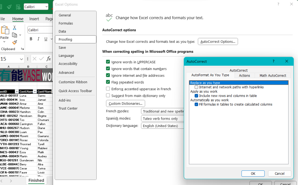
MedAttrib: author-generated. MS Excel default hyperlink option.
Individual Hyperlinks
When in a worksheet, you can select a cell that has an un-hyperlinked URL/email address in it, and make it active manually. We noted this in Chapter ___. To refresh:
- Select the needed cell A3.
- In the Inserts ribbon, click the Hyperlink button (near the middle right). There may be a list of recent documents you have used, but ignore those for now; click Insert Link which is listed at the bottom of the dropdown.
Insert Link will open an Insert Hyperlink panel, which offers the options to link to: “an existing file or web page”, a “place in the same workbook”, a “new creation of another document”, or “an email address”.
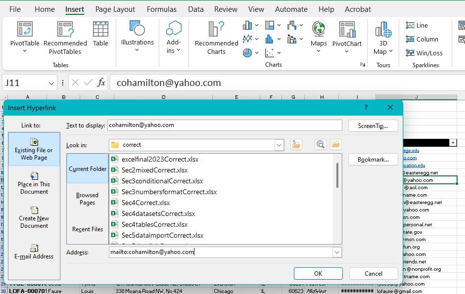
MedAttrib: author-generated. MS Excel Insert hyperlinks.
- Choose the Existing File or Web Page option.
- Then, in the Address field at the bottom of the panel, type the URL or Email address.
Keyboard Shortcut: Add Hyperlink. Hold down CTRL key while pressing letter K on your keyboard / Mac CMD K.
Function for Mass Hyperlinks
Sometimes, you may need to change a whole column of static text showing hyperlinks into active, clickable ones. There is a fairly basic function for that. Keep in mind that this will definitely be a formula using relative references – if you use a version to refer to specific cells.
HYPERLINK(link_location, [friendly_name])
- Link location (required) is the web page, email address, file location, or document anchor location.
- Friendly name (optional) is the name of the web page, or the person who owns the email, or the document being linked to.
Examples:
=HYPERLINK(“http://www.shoreline.edu”, “Shoreline Community College”)
=HYPERLINK(“#Sheet2!A1”, “Sheet2”)
=HYPERLINK(“C:\SCHOOL\BUS150\DataFiles\Links.xlsx”, “Excel Links File”)
=HYPERLINK(B2, A2)
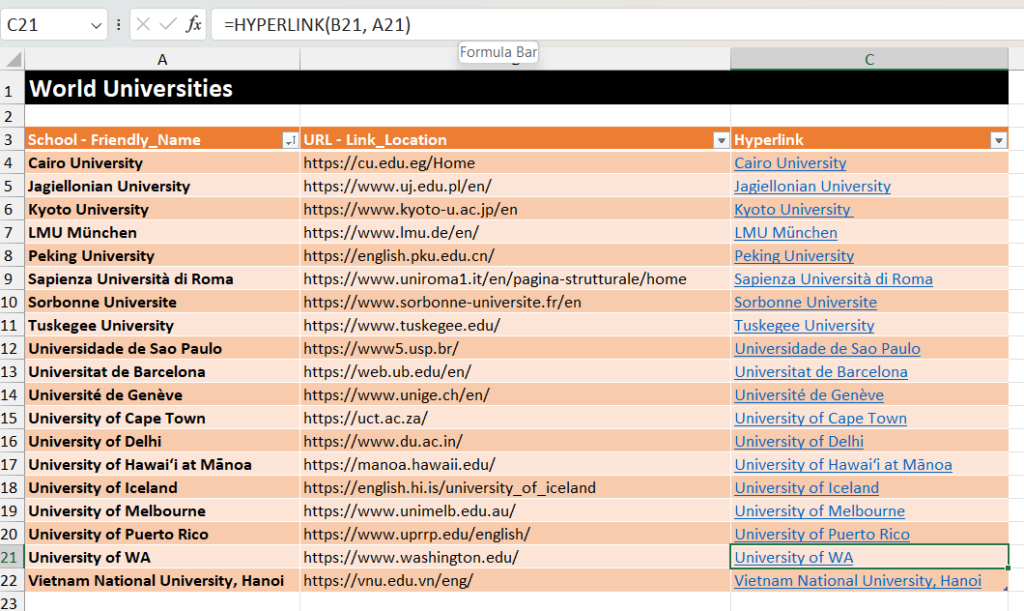
MedAttrib: author-generated. MS Excel mass hyperlinks.
NOTE: This is an example – if you want to practice, you can reopen the Ch14-Concat.xlsx file, and try this mass hyperlink formula for the emails in Column K. If you do, be sure create a new column in Column L, and call it something like EmailLinks, do the formula in there, and when finished to SAVE your file before closing it again.
Remove Mass Hyperlinks
This question here is whether to remove the clickable hyperlink, or the field altogether.
IF you want to remove the clickable hyperlinks in a column, you can select the whole column, copy it, then paste values over itself to keep only the text content, not the formula. This problem here is if you do this over a column in which all the hyperlink addressed are displayed as Friendly Names, the actual URL address will be stripped out of the cell when the formula is removed. So, ONLY use this on columns in which you can read the actual URL address.
