Chapter 16: Functions – Lookups / Logical

What We’ll Cover >>>

• VLOOKUP
• HLOOKUP
• XLOOKUP
• IF / nested functions

This chapter focuses mostly on lookup functions. We will also review a basic use of the IF function and a nested function.

The LOOKUP function is a built-in function in Excel that is categorized as a reference function. It can be used when you need to fill in some data in a dataset that is referenced in another dataset – in the same worksheet, another worksheet or another workbook. It isn’t as simple as using the Click Cell method to simply copy data from one place to another, because you might need to have to ask for the data to be found based on criteria in the existing dataset and where it is also referenced in another dataset. For example, you might you know the part number for a computer part in your dataset, and you need the price but your table doesn’t know it because it is listed in another table or dataset.

VLOOKUP

You need to use a VLOOKUP function to look up information in a table so that you can use that information in another table that needs it. It stands for Vertical Lookup, because the data is being looked up in reference to the columns of a table, not the rows. Is the information in a table’s column (default is yes, since most tables have their header rows for columns). If so, then you use a VLOOKUP.

There are four pieces of information (arguments) that you will need in order to build the VLOOKUP formula. These are the four arguments of a VLOOKUP function:

• The Lookup_value, which is the value you want to look up in the table you are inputting your formula into. This would be what your calculation cell needs from its own table to look up in another dataset for the answer.
• The Table_array is the range (table) where the lookup values and the values you want returned by the function are located.
• The Col_index_num, which is the column number in the data range that contains the value (information you need) to return to your calculation cell.
• The Range_lookup, which is your request for an exact match (false) or approximate match (true). It is best to use false so that your Lookup formula is exact.

TIP: LOOKUP Columns = 2. VLOOKUPs are tricky if you try to use them for anything other than looking in two columns of a table. They are linear in processing, so you need to use them for only 2 columns – the left column with the value that matches your Lookup_value, and the right column with the resulting data you want to be pulled over to your calculation cell. What if a lookup table has more than 2 columns? Easy! Just make a named data range of only the two columns you need to look in.

ACTION: Try Me activity

We will work with a combination activities workbook, named Ch16-Lookups.xlsx. Before you start working, go to your DataFiles folder and make a copy of the file for your Examples folder, then open that copy.

Our goal for our work has 3 parts, all of which are illustrated later in the chapter.

The workbook has two sheets; the first is named Lookups, and we can practice some of these functions with simple examples. The second is a static information sheet with some common lookup and logical functions you can use for your reference.

Go to the Lookups worksheet. On it is a table, called Movies, from cells A5-I19 with row 5 being the header row. Look at the empty cell D6. This cell needs to tell us what the Genre of the movie shown in cell B6 is. All we have is a Genre Code, though, and the actual Genre name is listed in another small table called Genre (Cells K6-L11) on the same sheet. How do we get that information into cell D6?

Here is what needs to happen. We need to tell cell D6 to look at cell C6 for the Genre Code. We then need to tell cell D6 to look that same Genre Code up in the Genre table of cells K6-L11, and tell us what the Genre Code in the K column represents from the L column. What????

D6 should look at C6, then look over at K column for whatever genre code matches and what its associated L column genre name is. Ummmm. . . okay.

Let’s try this:

VLOOKUP syntax:

• Calculation cell with the VLOOKUP formula = D6
• Lookup_value = C6
• Table_array = K6 – L11 (a 2-column data range)
• Col_index_num = 2  (which is the L column in a range of cells K6-L11)
• Range_lookup = FALSE (which means an exact match)
• Result = Adventure

So, here we go:

• Click Cell D6.
• Type =VLOOKUP([@GenreCode],Genre,2,FALSE)

Genre refers to the name of the 2-column table that makes up the 2-column dataset we needed to look in.

• Assuming your VLOOKUP worked and gave you Adventure in cell D6, IF Excel does not auto-populate D7-D19 with the formula, then copy the formula of D6 down through cells D7-D19.
• SAVE your work.

Let’s try another.

Click Cell F6. We want this cell to show the quality of the movie product. To do this, we will need to figure out where this information is. The 2-column Quality table lists the Quality codes and their respective quality label (fair, good, new).

Let’s use the function builder.

• In cell F6, click the FX symbol to the left of the Formula bar.

When the Function Arguments dialog box opens, do the following:

• In the Lookup_Value field, type in cell E6. Because this is in a named table, Excel interprets it as [@QualityCode]
• In the Table_Array, type Quality. OR, if you select the cell range of N6 – O9, make sure to make the reference ABSOLUTE in the function builder.
• In the Col_Index_Num, type 2, which is column 2 of the Quality Table_array we are looking in.
• In the Range_Lookup, type FALSE
• Click OK.

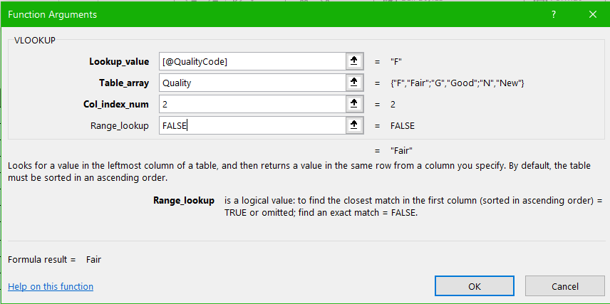
MedAttrib: author-generated. MS Excel VLOOKUP using Function Arguments dialog.

• Then, assuming you got a correct response in cell F6 (Fair), copy the formula of F6 down through cells F7-F19 if Excel does not auto-populate cells F7-F19 for you.

Click Cell H6. We want this cell to show the medium that the film is being sold on. To do this, you need to figure out where this information is. The 2-column Media table lists the Media codes and their respective medium (DVD, VHS, Blu-ray).

• You know what to do. Craft a VLOOKUP formula for H6. You can do it by hand or use the Function Arguments builder.
• Once you complete the formula accurately, copy the formula of cell H6 down through cells H7-H19 if Excel does not auto-populate those cells for you.
• SAVE your work.

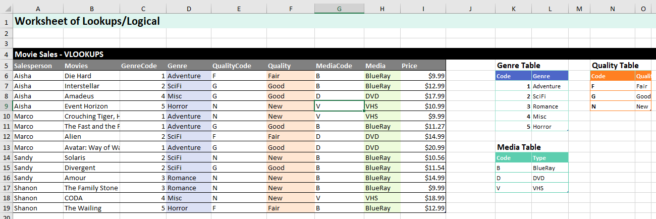
MedAttrib: author-generated. MS Excel VLOOKUPs activity.

Errors

Note: What if a VLOOKUP doesn’t work? What if we get a result different from the one predicted? In this case, we may have:

• Made a slight mistake entering the VLOOKUP function
• Tried to look in some other column instead of the second one in our data range
• Might not have named a data range at all if our data was in a Table_array that has more than 2 columns.
• The Lookup_value might not be in the Table_array

To make repairs in the function, click in the formula cell to activate it. In the Formula bar, press the Insert Function button. That will reopen the dialog box so you can make your repairs. Did you forget to make the cell references for the Table_array absolute (like a named data range or the $N$6:$O$9)? Did you use the wrong cell for the Lookup_value? Then, press OK when you are done reviewing the Function dialog box and recopy the corrected function down through the rest of the cells in the column.

HLOOKUP

You might need to use a lookup function to look up information in a table made up of rows (not columns) so that you can use that information in another table that needs it. HLOOKUP stands for Horizontal Lookup, because the data is being looked up in reference to the rows of a table, not the columns. Is the information in a table’s row. If so, then you use an HLOOKUP.

TIP: It is very important to specify a named range for the two rows you plan to look up your Lookup_Value in. HLOOKUPS can be a little sensitive without being clear as to why.

In this example, we are working with a table called Students of cells A24 – C29. We want to populate the Notes column with notes listed in the range of cells E24 – H25, which already has a Named Rage name of Comments. Our common information point between the two data ranges is the number of points a student received in the Students table, and the points that a specific note falls under in the Comments range.

HLOOKUP syntax:

• Calculation cell with the HLOOKUP formula = C25
• Lookup_value = B25
• Table_array = E24 – H25 (named Comments in the Formulas ribbon’s Name manager)
• Row_index_num = 2
• Range_lookup = FALSE
• Result = On Target

So, here we go:

• Click cell C25
• Type =HLOOKUP([@Points],Comments,2)

Comments refers to the name of the 2-row table that makes up the 2-row dataset we needed to look in.

• Copy the formula of cell C25 down through cells C26-C29, assuming your HLOOKUP worked and gave you On Target in cell C25.
• SAVE your work.

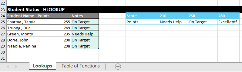
MedAttrib: author-generated. MS Excel HLOOKUP activity.

XLOOKUP

XLOOKUP is a fairly new lookup function in Excel, starting in 2021’s version/updates to MS Excel 365. Because of this, it is not backwards compatible with earlier versions of Excel. Many students and workers find themselves in workplaces that haven’t fully upgraded to current Office 365, and/or may be using other financial workbook tools from free and open-source providers.

XLOOKUP is able to search for data both horizontally and vertically while VLOOKUP searches only vertically and HLOOKUP searches only horizontally. It searches a range or an array, and then returns the item corresponding to the first match it finds. It can be considered a more elegant function, with only 3 arguments needed in most cases because the default match mode is 0 (exact match). However, it can be less intuitive to learn because it can have additional logical arguments which make the formula seem less than intuitive for new learners.

At this time, XLOOKUP is not being covered in this textbook, primarily because it is not backwards compatible. This may change as the function becomes more routinely used, and easier to interpret.

IF and Nested functions

IF Function

The IF function allows you to make a logical comparison between a value and what you expect by testing for a condition and returning a result of True or False. These decision results can be used to provide information, do different / additional calculations, and/or do further tests.

The IF function is one of the most popular functions in Excel. It allows you to make logical comparisons between a value and what you expect. In its simplest form, the IF function says something like:

IF the value in a cell is what you expect (true) – do this. If not (else) – do that. The IF function has three arguments:

• Logical test – Here, we can test to see if the value in a selected cell is what we expect. You could use something like “B7=14” or “B7>12” or “B7<6”
• Value_if_true – If the requirements in the logical test are met – like if B7 is equal to 14 – then it is said to be true. For this argument, you can type text – “True”, or another message like “On budget!” Or you could insert a calculation, like B7*2 (If B7 does equal 14, multiply it by 2). Or, if you want Excel to put nothing at all in the cell, type “” (two quotes).
• Value_if_false – If the requirements in the logical test are not met – if B7 does not equal 14 – then it is said to be false. You can enter the same instructions here as you did above. Let’s say that you type the double quotes here. Then, if B7 does not equal 14, nothing will be displayed in this cell.

Nested Functions

Nested functions are when a function needs to accomplish more than one thing, and needs the help or one or more functions added inside of its code. They allow you to test more than one thing in the same calculation,

For instance, a nested IF function is an IF function within another IF function. It might refer to something like:

• IF this, then that, else look this up, and IF this, then that, and. . .

You get the point. It is a calculation that behaves like a flowchart of choices and results.

In Ch16-Lookups.xlsx, we’ll continue working with the Lookups worksheet. We’ll do a simple IF function, and also a little more complex but fun nested IF function.

Cells A35 through E48 make up a table called Gens, including a header row. We need to do the formulas for column C to determine if the person in the record is an elder, and when we do the formulas for column E to determine if the person in the record is a GenX or Millennial, or in some other generation.

Click cell C36. We need to determine if Joah, who is age 26, is an elder. If his age meets certain conditions, then yes, Joah is an elder. If his age does not meet certain conditions, then no, Joah is not an elder.

Let’s use the function builder.

• In cell C36, click the FX symbol to the left of the Formula bar.

When the Function Arguments dialog box opens, do the following:

• In the Logical_Test field, type in B36 >64
• In the Value_if_true, type Yes
• In the Value_if_false, type No
• Click OK.

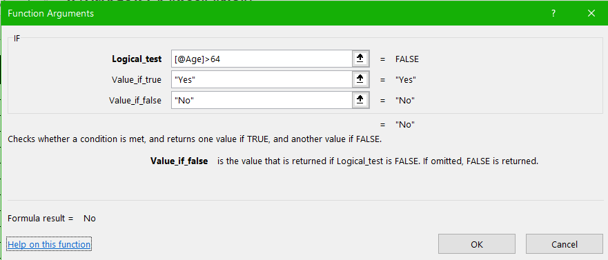
MedAttrib: author-generated. MS Excel IF activity in Function Arguments dialog.

This asks if the value of cell B36 (age 26) is greater than the age of 64. It is not greater, so cell C36 should return No.

• Copy the formula of cell C36 down into cells C37 – C48. (If Excel does not auto-populate the column for you.)
• SAVE your work.

Now, let’s find out what generation Joah is. Is he a GenXer? A Millennial? Or in some other generation? THIS is going to take sone doing, so hold on to yourself. . .

Basically, we have to ask:

If Joah’s birth year falls in a certain yearly range, he is GenX. If it does not fall into that range, then does his birth year fall into another yearly range? If yes, he is Millennial. If his birth year does not fall into that range, then he is some other generation.

This calculation takes some time to figure out, because it nests functions inside each other to ask and answer those things all in one cell. Plus, we have to look at Joah’s birth year in a range of dates, not just as one simple choice. This means we have to nest in AND functions, which has 2 arguments and Returns TRUE only if both of its arguments are TRUE.

• In cell E36, type =IF(AND(D36>1965,D36<1980),”GenX”,IF(AND(D36>1981,D36<1996),”Millennial”,”other generation”))

If Joah’s birth year in D36 is between 1965 and 1980, he is GenX, otherwise if his birth year in D36 is between 1981 and 1996, he is Millennial, otherwise he is other generation.

• Assuming that the function is satisfied that Joah is other generation (birth year 1997), we’re good.
• If Excel does not auto-populate the column for you, copy the formula in E36 down through cells E37 – E48.
• SAVE your work, and close the file. We’re done!

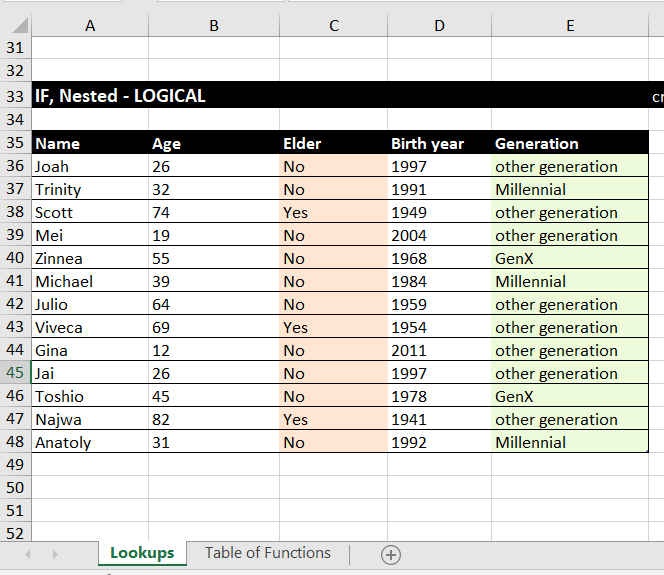
MedAttrib: author-generated. MS Excel IF and nested activities.