Chapter 2: Data Input / Editing

What We’ll Cover >>>

• Entering Data
• Editing Data
• Auto Fill
• Deleting Data
• Adjusting Columns/Rows
• Hiding and Unhiding Columns/Rows
• Inserting Columns/Rows
• Moving Data
• Deleting Columns/Rows

In this section, we will begin the development of a worksheet. The skills covered in this section are typically used in the early stages of creating one or more worksheets in a workbook.

Part of what we will cover here is inputting data. However, Excel can import data from other sources, like databases and other programs. We will look at data imports in Part 2. For now, we are simply getting used to the basics of Excel with more straightforward files and data input.

Let’s clarify what data in Excel actually means. The contents of any cell are referred to as the value in that cell – whether it is qualitative text or the quantitative returned information from a formula. Values in Excel include:

• Text: Plain text is static. It contains some combination of letters, numbers, spaces, and symbols. It is descriptive/informational, and in itself doesn’t provide the values of a formula. Text remains constant when it is used in a formula.
• Number: Numbers are data that is acted upon in formulas. They can be formatted to be different kinds of numbers, like currency, percentages, etc. They are what most formulas calculate with in order to give an answer and/or transform their meaning.
• Logical: Data in this type is either TRUE or FALSE, usually as the result of a test or comparison from a formula.
• Error: A value that returns if a formula cannot complete calculations properly.

Entering Data

Entering data in Excel is very unlike the type and enter experience you may have with word processing documents, presentation files, and web page text entry fields. Excel basically has to use information in little pieces in order to calculate with it, sort it, filter it, and otherwise analyze it. For instance, if you type a person’s name and address all in one line or worksheet cell, it can only be sorted by the very first letter, not the address, or zip code, or last name, etc.

This means that you will need to become comfortable with using cells, which is the medium with which Excel can identify pieces of data and use them.

Columns of cells tend to be referred to as fields of information. Rows of cells ten to be referred to as records of data. So:

• A person’s first name in a column is an entry in the column’s field. A column can have multiple fields (instances) of data, like a column of first names in a range of data. In the image below, Column A fields contain first names, like L.J., Alfre, Jonna, etc.
• A person’s row of information, like first and last name, email address, and favorite dessert, is a record for that one person. A data range is usually made up of many records. In the image below, the Row 1 record contains data like Ajay Bashira apple juice, etc.

ACTION: Try Me activity

• Follow along and try things. There is no “wrong”, this is just play and exploration!

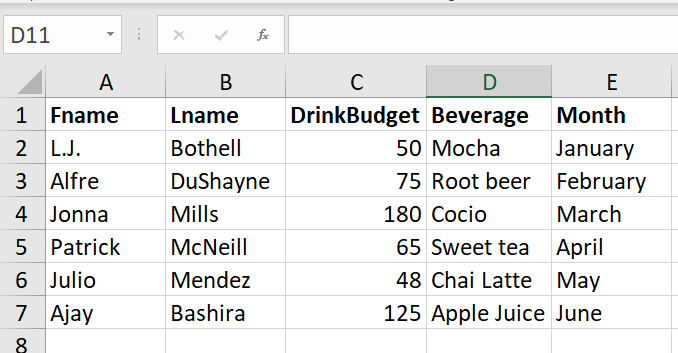
MedAttrib: author-generated. MS Excel cells, rows, and columns.

Plain Data

• BEFORE you do this activity, make sure you have taken the Preparation Steps in the Part 1 Introduction of this book – about creating file folders on your computer and downloading available files for later use. OR, if you have an instructor who requires other file folder organization and file naming standards, do that instead.  Either way allows you to have a safe place to save your files of work while you explore this content – your Examples folder.
• Once you have a storage space to save your work, Create a new, blank workbook in Excel.
• Immediately give it a name and save it to your chosen working directory folder on your computer. File naming recommendation: Ch2-DataEntry.xlsx.
• Click cell A2.
• Type your own first name in cell A2, then press the ENTER key. After you press the ENTER key, cell A3 will be activated. Using the ENTER key is an efficient way to enter data vertically down a column.
• Enter the following first names, pressing ENTER after each: A3=Alfre, A4=Jonna, A5=Patrick, A6=Julio, A7=Ajay
• Click cell B2.
• Type your own last name and press the ENTER key. After you press the ENTER key, cell B3 will be activated.
• Type the name DuShayne into cell B3 and press the ENTER key. Do this with the rest of the names through cell B7: Mills, McNeill, Mendez, Bashira
• Click cell C2.
• Type the number 50 and press the ENTER key.
• Enter the following numbers in cells C3 through C7: 75, 180, 65, 48, 125
• SAVE your work as you go: the Quick Access Toolbar shows a little disk icon, and the common keybind is CTRL S / Mac: CMD S.

MedAttrib: author-generated. MS Excel cells, rows, and columns.

TIP: Avoid formatting symbols when typing numbers. When typing numbers into an Excel worksheet, it is best to avoid adding any formatting symbols such as dollar signs and commas – just type in the numeric data itself. Although Excel allows you to add these symbols while typing numbers, it slows down the process of entering data. It is more efficient to later use Excel’s formatting features to add these symbols to numbers after you type them into a worksheet.

Column Headings

In Excel, data rarely means anything to a user if there is no context attached to it. Commonly this is done through column headings, which identify what the content in the column is supposed to be. This can also be done as row headers instead, but in this course we’ll mostly use the standard column headings.

In the image above, you likely also saw a row of bold text in cells A1-C1. These are column headers, and you can type them:

• In cell A1, type Fname, then press TAB. Tab lets you move to the right of an active cell and activate the next one to its right for data entry.
• In cell B1, type Lname and press TAB.
• In cell C1, type DrinkBudget, and press TAB.
• In cell D1, type FaveDrink, and press TAB.
• In cell E1, type Month and press TAB.

These are the column headings that tell you the first column is full of first name fields, the second column is full of last names, and the third column has amounts for a coffee budget, etc.

Editing Data

Data that has been entered in a cell can be changed by double clicking the cell location or by selecting the cell but typing data into the Formula Bar. You may have noticed that as you were typing data into an cell location (like A2), the data you typed also appeared in the Formula Bar. The Formula Bar can be used for entering data into cells as well as for editing data that already exists in a cell. The following steps provide an example of entering and then editing data that has been entered into a cell location:

• Click cell D2.
• Type Moc and press the ENTER key.
• Click cell D2 again to select it.
• Move the mouse pointer up to the Formula Bar. You will see the pointer turn into a cursor. Move the cursor to the end of the abbreviation Moc and left click.
• Type the letters ha to complete the word Mocha.
• Click the check mark to the left of the Formula Bar. This will enter the change into the cell.
• Use this method – clicking a cell but typing into it through the Formula Bar – to add coffee beverages you see in the Try Me image (above) into cells D3-D7.
• SAVE your work as you go: the Quick Access Toolbar disk icon, and keybind is CTRL S / Mac: CMD S.

Keyboard Shortcut: Editing Data in a Cell. Activate the cell that is to be edited and press the F2 key.

Auto Fill

The Auto Fill feature is a valuable tool when manually entering data into a worksheet. It is sometimes referred to as Smart Fill.  This feature has many uses, but it is most beneficial when you are entering data in a defined sequence, such as the numbers 2, 4, 6, 8, and so on, or nonnumeric data such as the days of the week or months of the year. It does not work for all seemingly consistent series – just for simple ones.

The following steps demonstrate how Auto Fill can be used to enter the months of the year in column E:

• Click cell E2 in the Sheet1 worksheet.
• Type the word January and press the ENTER key.
• Click cell E3 and type February, then Press Enter.
• Click cell E4 and type March, then Press Enter.
• Move the mouse pointer to the lower right corner of cell E4. You will see a small square in this corner of the cell; this is called the Fill Handle. When the mouse pointer gets close to the Fill Handle, the white block plus sign will turn into a black plus (+) sign.
• Left click and drag the Fill Handle down through cell E13. Notice that the Auto Fill tip box indicates what month will be placed into each cell. Release the mouse button when the tip box reads “December.”

Once you release the left mouse button, 12 months of the year should appear in the cell range E2:E13. You will also see the Auto Fill Options button. By clicking this button, you have several options for inserting data into a group of cells.

• SAVE your work as you go: the Quick Access Toolbar disk icon. Keybind is CTRL S / MAC: CMD S.

Deleting Data

There are several methods for removing data from a worksheet, and with each method, you use the Undo command if you change your mind. This is a helpful command in the event you mistakenly remove data from your worksheet.

You can delete data by selecting a cell and using your keyboard’s Delete button. You can right-click on a cell and choose Delete. You can select a cell and use the Home tab Editing group and choose the Clear icon, then Clear all.

• Select Cells E8 through E13.
• Press the DELETE key / Mac FN key + Delete. This deletes the contents of those cells.
• So that we can recover that information, click the Undo button – which is by default available in the Quick Access Toolbar. This should replace the data in the cells E8-E13.
• To re-delete the info, Use the Home tab Editing group and choose the Clear icon, then Clear all.

Keyboard Shortcut: Undo. CTRL key + Z key / Mac CMD key + Z key.

Adjusting Columns/Rows

TIP: Column and Row Addresses. Every row has an address – the gray “cell” number to the left of the editable part of your worksheet. Every Column has one too, the gray “cell” letter just above the editable part of your worksheet. You click on these to select a whole row or column.

There may be a few entries in a worksheet that appear cut off. This is because the column is too narrow for the contents. The columns and rows on an Excel worksheet can be adjusted to accommodate the data that is being entered into a cell using  different methods. The following steps explain how to adjust the column widths and row heights in a worksheet.

• Bring the mouse pointer between column A and column B in the Sheet1 worksheet. You will see the white block plus sign turn into double arrows.
• Click and drag the column edge to the right so the entire column looks like it is about 2 inches wide. As you drag the column, you will see the column width tip box. This box displays the number of characters that will fit into the column using the Calibri 11-point font which is the default setting for font/size.
• Release the left mouse button.

You may find that using the click-and-drag method is inefficient if you need to set a specific character width for one or more columns. This is a second method for adjusting column widths when using a specific number of characters:

• Click any cell location in column A by moving the mouse pointer over a cell location and clicking the left mouse button. You can highlight cell locations in multiple columns if you are setting the same character width for more than one column.
• In the Home tab of the ribbon, left click the Format button in the Cells group.
• Click the Column Width option from the drop-down menu. This will open the Column Width dialog box.
• Type the number 29 and click OK on the Column Width dialog box. This will set column A to this character width.

A third method is the double-click one:

• Once again bring the mouse pointer between column A and column B so that the double arrow pointer displays ,and then double-click to activate AutoFit. This features adjusts the column width based on the longest entry in the column.

Row Height adjustment works similarly. Steps 1 through 4 demonstrate how to adjust row height, which is similar to adjusting column width:

• Click cell A1.
• In the Home tab of the ribbon, left click the Format button in the Cells group.
• Click the Row Height option from the drop-down menu. This will open the Row Height dialog box.
• Type the number 24 and click OK on the Row Height dialog box. This will set Row 1 to a height of 24 points. A point is equivalent to approximately 1/72 of an inch. This adjustment in row height was made to create space between the totals for this worksheet and the rest of the data.

Now, to adjust the row with the autofit option:

• Bring the mouse pointer between row 1 and row 2 so that the double arrow pointer displays, and then double-click to activate AutoFit. This features adjusts the row width based on the largest entry in the row.
• SAVE your work as you go: the Quick Access Toolbar disk icon, and keybind is CTRL S / Mac: CMD S.

Keyboard Shortcut: Column Width. Hold ALT key then press letters H, O, and W one at a time. Mac Users: not available.

Keyboard Shortcut: Row Height. Hold ALT key then press letters H, O, and H one at a time. Mac Users: not available.

Hiding and Unhiding Columns/Rows

In addition to adjusting the columns and rows on a worksheet, you can also hide them. This is a useful technique for enhancing the visual appearance of a worksheet that contains data that is not necessary to display but which is otherwise needed for computations and/or storage.

• Click cell C1.
• Click the Format button in the Home tab of the ribbon.
• Place the mouse pointer over the Hide & Unhide option in the drop-down menu. This will open a submenu of options.
• Click the Hide Columns option in the submenu of options. This will hide column C.

To unhide a column – like the now hidden column C – follow these steps:

• Select the columns B and D, which now seem to be right next to each other.
• Click the Format button in the Home tab of the ribbon.
• Place the mouse pointer over the Hide & Unhide option in the drop-down menu.
• Click the Unhide Columns option in the submenu of options. column C should now be visible on the worksheet.

Keyboard Shortcut: Hiding Columns. Hold down CTRL key while pressing the number 0 on your keyboard.

Keyboard Shortcut: Unhiding Columns. Highlight cells on either side of the hidden column(s), then hold down CTRL key & SHIFT key while pressing the close parenthesis key ). MAC: Hold down Control and Shift keys and press the number 0.

The following steps demonstrate how to hide rows, which is similar to hiding columns:

• Click row 3.
• Click the Format button in the Home tab of the ribbon.
• Place the mouse pointer over the Hide & Unhide option in the drop-down menu. This will open a submenu of options.
• Click the Hide Rows option in the submenu of options. This will hide row 3.

To unhide a row, follow these steps:

• Select the rows 2-4, which will seem to be right next to each other.
• Click the Format button in the Home tab of the ribbon.
• Place the mouse pointer over the Hide & Unhide option in the drop-down menu.
• Click the Unhide Rows option in the submenu of options. Row 3 will now be visible on the worksheet.

Keyboard Shortcut: Hiding Rows. Hold down CTRL key while pressing number 9 key on your keyboard.

Keyboard Shortcut: Unhiding Rows. Highlight cells above and below the hidden row(s), then hold down CTRL key & SHIFT key while pressing the open parenthesis key ( . MAC: Hold down CTRL + SHIFT keys and press the number 9.

TIP: Hidden Rows and Columns. In most careers, it is common for professionals to use Excel workbooks that have been designed by a coworker. Before you use a workbook developed by someone else, always check for hidden rows and columns. You can quickly see whether a row or column is hidden if a row number or column letter is missing.

Inserting Columns/Rows

Using Excel workbooks that have been created by others is a very efficient way to work because it eliminates the need to create data worksheets from scratch. However, you could realize that to accomplish your goals, you may need to add additional columns or rows of data. In this case, you can insert blank columns or rows into a worksheet. The following steps demonstrate how to do this:

 

 

 

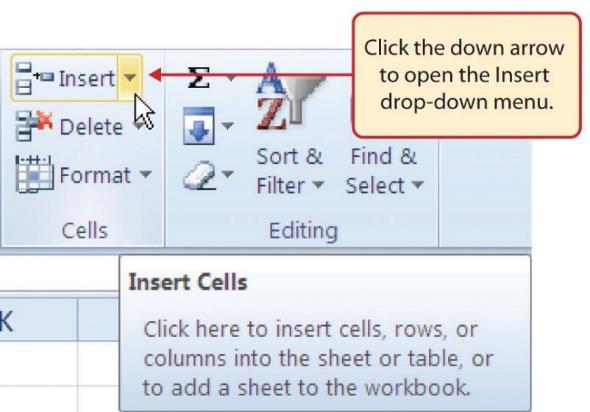
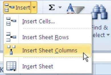
MedAttrib: Beginning to Intermediate Excel. MS Excel Insert Drop-Down Menu.

To insert a row with the same kind of process:

• Click cell A3.
• in the Home tab of the ribbon, click the down arrow on the Insert button.
• Click the Insert Sheet Rows option from the drop-down menu. A blank row will be inserted above row 3. The contents that were previously in row 3 now appear in row 4. Note that rows are always inserted above the activated cell.
• SAVE your work as you go: the Quick Access Toolbar disk icon, and keybind is CTRL S / Mac: CMD S.

Keyboard Shortcut: Inserting Columns. Press the ALT key and then letters H, I, and C one at a time. MAC: First hold down the Control key and press the spacebar to select the column; then hold down the Shift and Controls keys and press the + symbol.

Keyboard Shortcut: Inserting Rows. Press ALT key and then letters H, I, and R one at a time. MAC: First hold down Shift key and press spacebar to select row; then hold down Shift & Controls keys and press the + symbol.

Moving Data

Once info is entered into a worksheet, you have the ability to move it to different locations. The following steps demonstrate how to move data to different locations on a worksheet:

• Select the data range cells A1-D7.
• Bring the mouse pointer to the left edge of cell D2. You will see the white block plus sign change to cross arrows. This indicates that you can left click and drag the data to a new location.
• Left Click and drag the mouse pointer to cell D2.
• Release the left mouse button. The data now appears starting in column D, rather than in column A where it previously was.
• Click the Undo button in the Quick Access Toolbar (or use Ctrl+Z keyboard shortcut). This moves the data back to where it started in cell A1.
• SAVE your work as you go: the Quick Access Toolbar disk icon, and keybind is CTRL S / Mac: CMD S.

TIP: Moving Data. Before moving data on a worksheet, make sure you identify all the components that belong with the series you are moving. For example, if you are moving a column of data, make sure the column heading is included. Also make sure you grab all of the data in the range, so you don’t leave something out.

Deleting Columns/Rows

You may need to delete entire columns or rows of data from a worksheet. This need may arise if you need to remove either blank columns or rows from a worksheet or columns and rows that contain data. The methods for removing cell contents were covered earlier and can be used to delete unwanted data. To delete a column:

• Click cell C1.
• in the Cells group in the Home tab of the ribbon, click the down arrow on the Delete button.
• Click the Delete Sheet Columns option from the drop-down menu. This removes column C and shifts all the data in the worksheet (to the right of Column B) over one column to the left.
• Click the Undo button in the Quick Access Toolbar (or Ctrl + Z). This returns the column you deleted.

The same process works for deleting and undeleting a row:

• Click cell A3.
• In the Cells group in the Home tab of the ribbon, click the down arrow on the Delete button.
• Click the Delete Sheet Rows option from the drop-down menu. This removes row 3 and shifts all the data (below row 2) in the worksheet up one row.
• Click the Undo button in the Quick Access Toolbar (or use Ctrl+Z keyboard shortcut). This returns the row you deleted.

Keyboard Shortcut: Deleting Columns. Press ALT key and then letters H, D, and C one at a time. MAC: Hold down Control key and press spacebar to select column; then hold down Control key & press the – symbol.

Keyboard Shortcut: Deleting Rows. Press ALT key and then letters H, D, and R one at a time. MAC: Hold down Shift key and press spacebar to select row; then hold down Control key & press the – symbol.

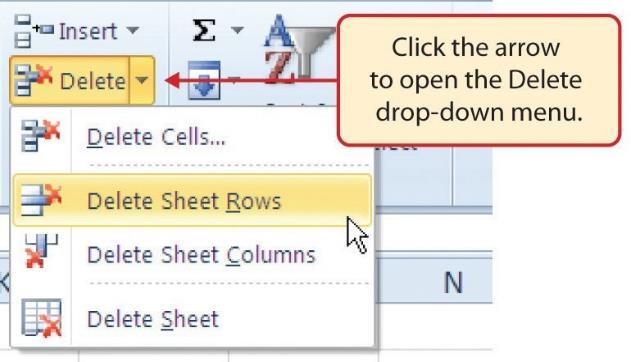
MedAttrib: Beginning to Intermediate Excel. MS Excel Delete Drop-Down Menu.

FINISHED!

• SAVE your work by clicking either the Save button on the Home ribbon; or by selecting the Save option from the File menu, or the Quick Access Toolbar disk icon, or the keybind CTRL S / Mac CMD S.