Chapter 6: Distribution

What We’ll Cover >>>

• Print Preview
• Page Layout
• Repeating Column/Low labels
• Page Breaks
• Print Area
• Headers and Footers
• Spell Checker
• Cleanup with Find & Replace
• Accessibility Review
• Notes and Comments
• Protecting Workbooks and Worksheets
• Backstage Info Page
• Distribution Methods

Excel workbooks can be distributed in several ways, such as a printed document, a PDF for printing or adding to a website, shared in the cloud through OneDrive, linked into a SharePoint site, and exported to PowerBI (a business enterprise application). Whatever method you might need to use to share your workbooks, setting them up for readability, printability, and clear defining between pages and sections is important. For our purposes, we’ll focus on practical standards for printing, which also translate well to PDFs and to being linked into a SharePoint (because other people might print or view your workbook(s) in a meeting, etc.)

ACTION: Try Me activity

Please find and open CH6–Distribute.xlsx, and save a copy to your Examples folder. Some of our work will use the Page Layout menu ribbon, with some coverage of the Review menu ribbon, and some coverage of the Home menu’s Backstage area for Info, Print, Share, Export, and Publish.

Print Preview

Print previewing may seem to be an odd place to start a chapter on distributing Excel workbooks, since there are a lot of pre-distribution tasks one needs to get done first. However, Print previewing is also the quickest way to see how a document will look when you print it, so we’ll start here.

With CH6–Distribute.xlsx open, go to your File menu item on the menu bar. When you click File, you will enter the Excel Backstage area (covered in Chapter 1). Much of the Backstage area has to do with printing and other document distribution options.

• In the Backstage area, click Print.
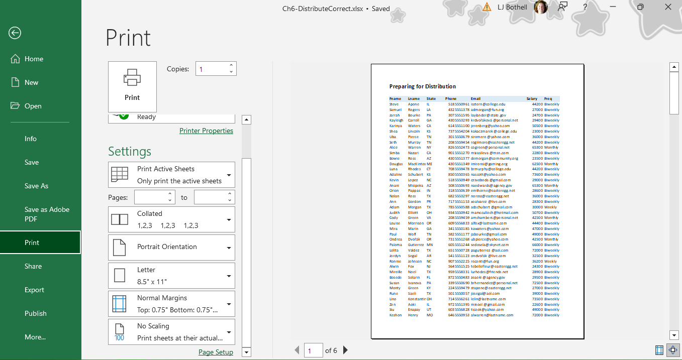
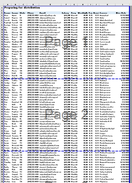
• Look at how the CH6-Distribute.xlsx will look if we just printed it as is. Below the image of the page printout, there is a field that reads Page 1 of 6. The data would be there, but it would be messy, with confusion as to which page is which.

Keyboard Shortcut: Print (and Print preview). CTRL key P / Mac CMD P.

In this view, the left hand side of the Print preview page tells us what the page size, orientation, margins, page scaling for print, and which sheets will be printed. The information shown in the Print preview page is the default for Excel, and you’ll need to make changes.

The Print preview page can be used for making changes to your document if you need to do so just before printing. For instance, a common adjustment is to choose to print the full workbook (all worksheet tabs, not just the current one you were on before going to the Print preview). Another common adjustment is the scaling of the page on the printout. The Collated/Uncollated option has to do with how a printer (particularly an office printer with many options) will output your documents.

However, while you can use the Print Preview page to change margins, page orientation, and page size, this is a messy use of your time. Planning those things should happen as you begin a new document, the same as the Theme (Chapter 6) and other page layout options (see below).

TIP: No printer? Many people do not have a printer accessible where they work (home, in a classroom, in a coffeeshop or at a friend’s home, etc. In this case, some of your prep work may not work if Excel doesn’t recognize a printer to address options to. Easy fix: Set your printer to “Microsoft Print to PDF”, which acts as a virtual printer structure.

Instead, we’ll focus on the Page Layout menu ribbon for common workbook and worksheet setup.

MedAttrib: author-generated. MS Excel Print preview.

Page Layout

For any document you work on – Word, PowerPoint, and Excel – you need to plan your output even as you are creating a new document. You will likely inherit a lot of workbooks in the workplace and need to contend with what you receive, and even then it is a good practice to understand a document’s shape and size before getting into the actual content.

The Excel Page Layout menu ribbon offers most tasks you need to accomplish to set your documents up appropriately to your needs. What you do here will stick with your document and once in the Print preview before printing/distributing your work, the prepared output should be assured. Note that your changes will affect only one sheet of your workbook unless you temporarily group them.

TIP: Multiple Worksheet set-up: You can select all the worksheets in your workbook and set the Page Layout options all at once, if you know what your project parameters will be.

• With your CH6-Distribute.xlsx file open, select both the Distribution sheet and Sheet2 by clicking on the Distribution sheet worksheet tab, holding the SHIFT key down, and then clicking on the Sheet2 worksheet tab.
• Go to the Page Layout ribbon’s Page Setup group, and click Margins.
• With Margins open, choose Narrow. Then, click Margins again, and choose Custom Margins (at the bottom).
• Custom Margins will open the Page Setup panel, and the Margins tab in it. Make the changes to the margins that you see in the image below:
• Top margin=1,   Bottom margin=.70,   Header=.25,   Footer=.25,   Center on page=Horizontally

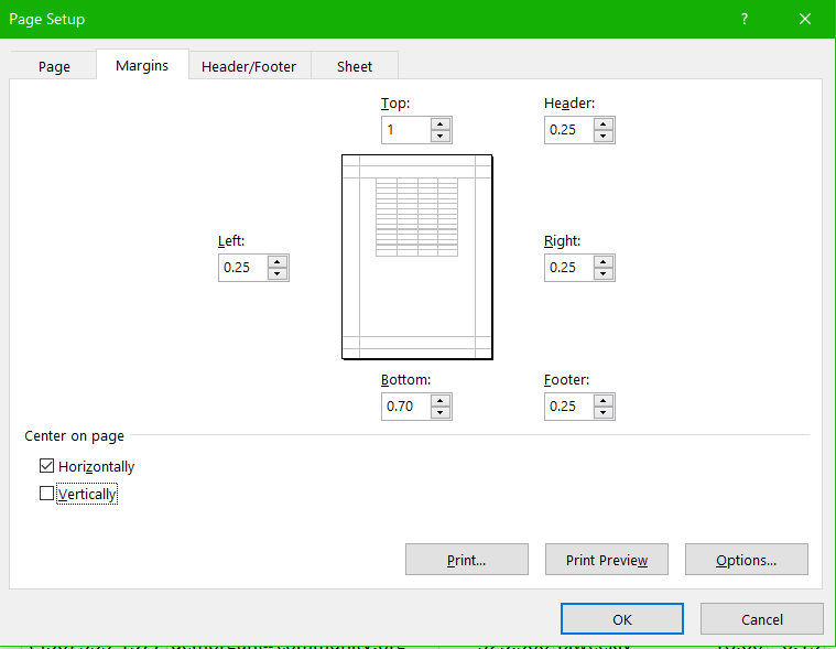
MedAttrib: author-generated. MS Excel Page setup.

• Click OK to exit the Page Setup panel.
• Next, with both the Distribution sheet and Sheet2 still selected together, choose Orientation from the Page Layout ribbon’s Page Setup group.
• Choose Landscape. The default is Portrait, which makes the worksheet print-out taller than it is wide. Landscape will make it wider than tall, and help accommodate more columns of information on the same page.
• With both the Distribution sheet and Sheet2 still selected together, choose Size from the Page Layout ribbon’s Page Setup group.
• In the Size dropdown, choose Legal. Legal (8.5″ x 14″) is often used for spreadsheets due to their many columns that need to appear on a single page.
• If you do not see that, or if some/all of the options in page size are grayed out, you may not have Excel recognizing a printer – or you may not even have a printer. In this case, you can use the tip from the Print Preview section above to set a printer as “Microsoft Print to PDF”.
• Check how the page will look using the File menu’s Backstage Print preview page. Now when you look, all the columns appear on the same page instead of being broken up. You can also observe that the first three ‘pages’ to be printed are from the Distribution worksheet, and the 4^th page is for Sheet2.
• SAVE your work as you go: Keybind is CTRL S / Mac CMD S.

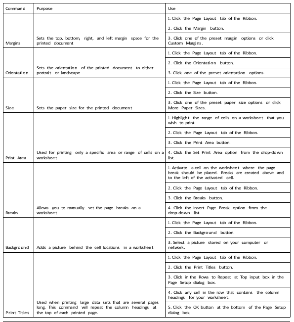
MedAttrib: Beginning to Intermediate Excel. Purpose and Use for Page Setup Commands.

Repeating Column/Row Labels

One significant problem exists for what we see in the Print preview. The Distribution worksheet has 3 pages, but only the first page shows the header row, which makes interpreting the second and third page difficult,

Now that you have fixed the cell and text formatting, you are ready to review the worksheet in Print Preview. You will notice that the worksheet is printing on multiple pages, and you cannot tell what each column of data represents on some of the pages.

• With CH6–Distribute.xlsx open, select ONLY the Distribution worksheet tab by clicking on it; this should ‘ungroup’ the previous both-worksheets selection.
• On the Page Layout ribbon’s Page Setup group, click the Print Titles button. The Page Setup panel will open to the Sheet tab.

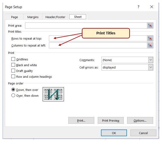
MedAttrib: Beginning to Intermediate Excel. MS Excel Page Setup Sheet panel

• Click in the Print Titles / Rows to repeat at top field. Be sure your insertion point is blinking in that box before moving on to the next step.
• In the worksheet, select Row 3. The text $3:$3 should now appear in the Rows to repeat at top field.
• While still in this panel, also choose Page Order: Over, then down. While we hope that all out columns will stay on one “page”, of they do overflow it would be easier to sort if the tag-end page printed just after its main page, rather than at the end of the print session.
• Go to Print Preview (CTRL P) and look at each of the pages. Notice that the first three rows are now repeated at the top of each page.
• SAVE your work.

You will not see a change to the worksheet in Normal view, so you will need to return to Print Preview. In our case, this seems to be good enough, but in other documents, you may find that pages are breaking in inconvenient places, such as when some cells are word wrapped. We’ll continue good standard practices as if this were the case.

Page Breaks

If data is split between pages, you may want to set a page break to force Excel to push a row down to the next page to avoid orphaning some visual data. We want all of the data for each state to be together on the same page for better analysis, so we need to control the page breaks. We are going to start by inserting a page break before the data in Row 25 to force Row 25 to start on the next page.

• With your cursor anywhere in your Distribution worksheet’s workspace, go to the View menu ribbon, and in the Workbook Views Group click then click Page Break Preview.

MedAttrib: author-generated. MS Excel Page Break Preview.

Mac Users: in the next paragraph, the location of the automatic page breaks may be in different locations. That’s ok.

In Page Break Preview, automatic page breaks are displayed as dotted blue lines. These lines indicate where Excel will start a new page. For this worksheet, we want the first page to break before Row 25 with Cody Green’s name, so we are going to insert a manual page break.

MedAttrib: author-generated. MS Excel Page Breaks Button on Page Layout tab.

• Select cell A25. When inserting a page break, you select the cell below where you want the page break to appear.
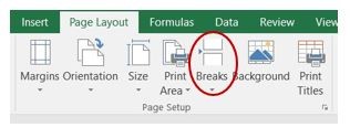
• Select the Page Layout ribbon and then click the Breaks button in the Page Setup group.
• Select Insert Page Break from the menu. There is now a solid blue line after row 24, which indicates a manual page break that was inserted.
• Do the same thing just above cell A50, and cell A75.
• Go to Print preview (CTRL P). Notice that we now have 4 pages on this worksheet for printing.
• Exit the Backstage area and then SAVE your work.

Print Area

Setting a print area for your workbooks is another standard practice. Even though this CH6–Distribute.xlsx file seems to look good, we are going to set a print range that leaves out the Hire Date. We don’t want to delete that column, and hiding it doesn’t always work for print/distribution needs.

• Select Cells A1–K90. This is the only part of the worksheet that you want to have print.
• On the Page Layout ribbon, click the Print Area button. Choose Set Print Area from the menu.
• Preview the worksheet in the Print preview page (CTRL P) to check that the print area that leaves out the Hire Date column setting worked.
• SAVE your work.

Headers and Footers

When printing worksheets from Excel, it is common to add headers and footers to the printed document in order to show on every page important information like the date, page number, file name, company name, and so on. Headers and footers show up on every page in Print preview and in print pages, even though you won’t see them in Normal worksheet view.

• Go to the Insert ribbon and click on the Text button near the top right.
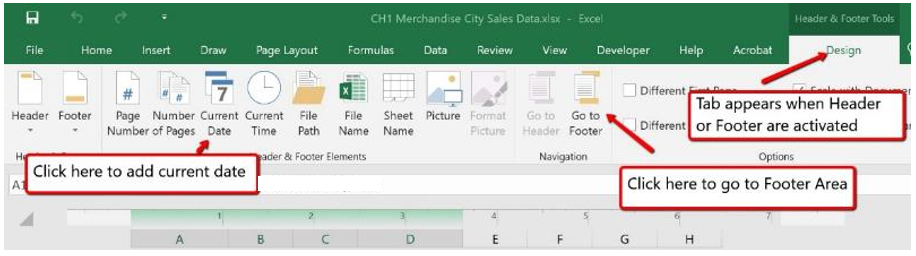
• Click on Header & Footer button. This will add a contextual Header & Footer menu ribbon with various options to add to your document. Also, this will convert the view of the worksheet from Normal to Page Layout. This Page Layout view makes adding Headers & Footers easy and provides key features to incorporate.
• In the opened Header space, click inside the left header section to edit the field.
• Click on the Current Date icon on the ribbon to add the date to the left section of the worksheet Header. The &[Date] symbols which will toggle to a Date format when you click outside of this area.

MedAttrib: Beginning to Intermediate Excel. MS Excel Design Tab for Creating Headers and Footers.

• In the Header section, click inside the middle header section to enter the field, then type your name in it.
• Click the Go to Footer button in the Navigation group of commands in the Design tab of the ribbon.
• Place the mouse pointer over the far right section of the footer and click to edit the field.
• Click the in the Header & Footer ribbon, choose the Page Number button in the Header & Footer Elements group. This view will display as &[Page] until printed or until you return to normal view.
• Click any cell location outside the header or footer area. The tab and ribbon for creating headers and footers will disappear.
• Click the Normal view button in the Excel Status Bar’s lower right side.
  • Or, you can instead choose the View menu ribbon, and in the Workbook Views group click the Normal view.

• SAVE your work.

Spell Check for Corrections

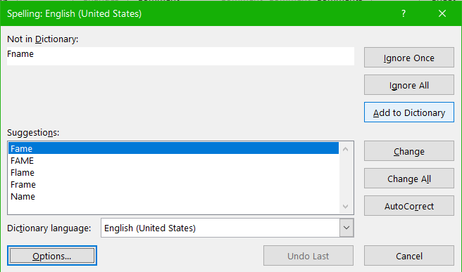
Before you distribute your workbooks, it is good standard practice to check them for spelling errors. This can be tricky in workbooks with a lot of customer names, and addresses with unique spellings. However, there is no substitute for spell checking when your work needs to be proficient and clean.

With the spell check / editor, you can go through Excel’s selected misspellings one at a time to determine if you want to keep the existing item, or to make changes to it. Excel will offer options, or you could click into the worksheet where the misspelling appears and manually change it. You can ignore it once or ignore all.

Keyboard Shortcut: Spell Check. Press the F7 function keyboard button.

MedAttrib: Beginning to Intermediate Excel. MS Excel Spell Checker.

Accessibility Review

Another standard practice is to check the accessibility of your workbook content before you release it. The Accessibility Checker is a tool that reviews content and flags accessibility issues it encounters. It notes why each issue might be a potential problem for someone with a disability, and also suggests how you can resolve the issues.

The default setting is for the Accessibility Checker to run in the background while you work.

• Select the Review ribbon’s Check Accessibility icon, then to manually launch the Accessibility checker. This will open an Accessibility contextual ribbon, as well as a docked Accessibility panel that shows specific issues.
• In our CH6–Distribute.xlsx file, the only accessibility issue seems to be that the second worksheet is named Sheet2. An explanation is given in the panel.

Other things the Accessibility checker might reveal in varying worksheets include:

• Images, icons, shapes, WordArt, SmartArt, and other graphic elements that need Alt text added to them for screen readers.
• Tables, including header rows, table names. Excel default to to names like Table1, Table 2, etc., which can be confusing for people relying on screen readers and which should be named specifically for the purpose and work they are used for in the document. Example: Table1 should be renamed to something like SalesRepRegions.
• Issues with color contrasts that the checker might pick up in custom conditional formatting or text/cell styling.
• You can check the Microsoft® support pages for information on making Excel documents accessible.

Notes and Comments

Before you release your work, especially if it is going to colleagues who are also working on a project related to the workbooks, you might want to add notes or comments to a worksheet.

Notes are for adding annotations in cells, like a reminder, and they don’t have any interaction. Comments are used if you are working with others and want to interact in the document to discuss data and analysis. Each can be inserted by using the Review menu ribbon. Let’s make a comment in our CH6–Distribute.xlsx file’s Distribution worksheet.

• Click on cell E1, since this seems to be a nice, central open area where a comment could be easily seen.
• In the Review ribbon’s the Comments group, choose New Comment.
• When the comment panel opens, type the following into the text field: Let’s consider deleting the Sheet2 since it duplicates some information from the Distribution sheet.
• Then, click the green Enter arrow in the comment panel. The comment itself will not show, but in the upper right corner of the cell E1, a little flag is attached. It can be hovered over to view and reply to the comment.
• SAVE your work.

Protecting Workbooks and Worksheets

If you need to protect the data in your workbooks from being edited, you can easily protect the full workbook, protect specific sheets, and open only specific ranges of data to editing.

There are two places you can choose from to manage your protections:

• The Review menu ribbon’s Protect group, and
• The Backstage’s Info page.

For this activity, we’ll work with the Review menu.

• In our file, choose Sheet2.
• Choose the Review ribbon, then the Protect group.
• In the Protect group, click Protect Workbook. When you click that, you’ll see a dialog box that asks for a password. When you do this, assign something you will remember. We will not do this task.
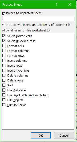
• In the Protect group, click Protect Worksheet. This will protect only the worksheet named Sheet2, which you should still be in. This will open a more detailed Protect Sheet panel. The two top items are already checked by default, which means that users of the worksheet will only be able to select locked and unlocked cells.
• In our activity, let’s give users the ability to also sort the worksheet’s data by checking the Sort checkbox.
• Then, enter the word password (all small letters) in the Password field. If asked to re-enter the password, use the same one.
• Click OK.
• Click on cell A1, and attempt to delete the contents. You should see a warning message that the worksheet is protected.
• Click on the worksheet tab for Distribution to go to your main sheet.
• Then, choose the Review ribbon’s Allow Edit Ranges icon, which will open the Allow Users to Edit Ranges panel.
• In the Edit Ranges panel, click New to set a specific range to allow to be edited with a password.
• In the ‘Title’ text field input Taxes. In the ‘Refers to cells’ text field, input =I4:I90 (that is a capital I, not the number 1). In the Range password field, input okay (all small letters). Then click OK.
• When you click OK, the Allow Edit Ranges panel should show that you have one range that allows editing by users if they have the password. Click Apply.
• Before you exit this panel, you still need to protect this worksheet. At the bottom left of the panel, click Protect sheet. In the resulting Protect Sheet panel’s password field, input password (all small letters). Click Apply, then OK to exit the Protect sheet.
• Click OK again to exit the Allow Edit Ranges panel.
• Now, if you try to edit any cell in the Distribution workbook, you will get the protection message. If you try to edit any of the numbers in the Taxes column, you will be offered the chance to give the password to edit the information.
• SAVE your work.

MedAttrib: Beginning to Intermediate Excel. MS Excel Protect Worksheet panel.

Backstage Info Page

• With all these steps and considerations, you’d think we’d be done, right? Well, there is one more thing you should be aware of: the Excel Backstage Info page. The Info page is a section gives you an overview of information about your document: its properties, its version history, browser view options, a place to inspect for any issues prior to distributing it, and the document’s protection/locked status.
• Let’s see what CH6–Distribute.xlsx has for us to know.
• Choose File to get to the Excel Backstage (PC for windows).
• Then, click the Info icon on the left-side. This takes you to the Info page.
• 

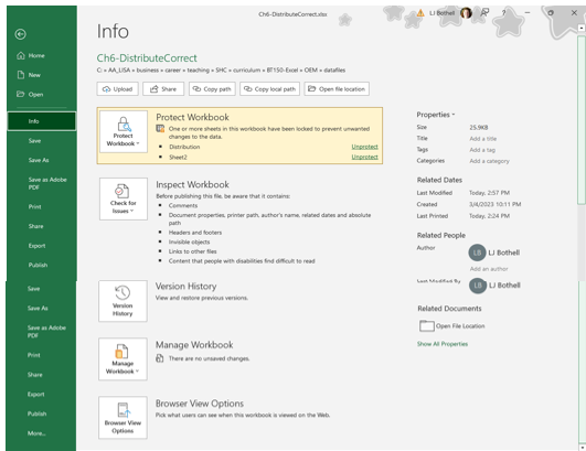
MedAttrib: author-generated. MS Excel Backstage Info page.

From this, we can see the name of the CH6–Distribute.xlsx file and its location on my computer. We can see that I am the author and editor of this workbook and the modification dates. When YOU look at YOUR copy, your own name should be listed at the Last Modified By information because you have been making changes to the original document for this activity.

In Properties, we also see blank fields, which are for metadata that would be built into the documents coding and would stick with it when the document is uploaded, saved as a PDF, etc. Let’s fix these.

• Under the Properties heading, click in the Title field, and input: Bootcamp Distribute example file
• In the Tags field, type your own name, and also the words/phrases Excel Bootcamp file, printing, accessibility, workbook layout. Each phrase should be separated by a comma.
• In the Categories field, type input Education, OER, Excel. Each phrase should be separated by a comma.
• Near the bottom of the Properties area, under the Related Documents heading, click the link See All Properties. This will expand the Properties info area. We don’t need to add anything to the Properties although in the Subject field, we could add Excel learning.

Now, look at the Protect Workbook information. After our tasks above, you should see that each worksheet (Distribution, Sheet2) is protected. You could change that here.

• Click the Protect Workbook “Unprotect” link beside the reference to Sheet2. In the dialog box asking for your password, type the one you chose.  This will unlock that sheet. Note how after this, the Protect Workbook section shows only one protected worksheet: Distribution.
• Look at the Inspect Workbook section. This lists some things to be aware of, like “Content that people with disabilities find difficult to read.”
• Click the Check for Issues icon. This offers the Check for Accessibility task we already reviewed above, and also Check for Compatibility.
• Click Check for Compatibility. The image below shows the resulting Compatibility Checker panel, expanded. You have the choice to select all or only a couple of versions of Excel in the Select Versions to Show dropdown. The summary of issues shows what the issues are, what their impact might be, and which version of Excel they stem from.
• Click OK to exit the checker.
• SAVE your work.

TIP: Expanding open panels/dialog boxes. If you see a small diagonal triangle at the lower right corner of an open panel or dialog box, this means you can click on that triangle and drag your cursor to enlarge the panel for more viewability of the content.

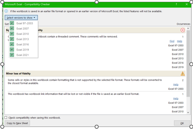
MedAttrib: author-generated. MS Excel Compatibility Checker panel.

Distribution Methods

Excel has many ways you can distribute your work:

• Printed document.
• PDF for printing or adding to a website.
• Shared document in the cloud through OneDrive.
• Linked into a SharePoint site.
• Exported to PowerBI (a business enterprise application).
• Exported as content into a database or other spreadsheet.
• Linked to a Word or Excel document (such as for graphs in a PowerPoint. presentation.

Whichever you need or choose, having your work properly formatted for layout helps other people experience and analyze the information. Checking for accessibility and compatibility helps catch and remove barriers for other users who need screen readers, have visual color issues, etc. Protecting data worksheets that you want viewed but not edited helps keep the worksheet’s content integrity.

With CH6–Distribute.xlsx open, go to the File/Backstage area and look at the options for distribution. The Backstage lists several, but the same task(s) can be accomplished in more than one of those areas, like print to PDF, export to PDF, save as PDF, etc.

• You can SAVE your workbook.
• You can Save As your workbook – save it as a different version of Excel, a CSV (comma delimited format), as a PDF, or as another type. You can save it to a different location.
• You can print the workbook and make printing-level changes, such as which specific sheets to print, collated or not, and scaling changes to fit the paper available.
• You can share the workbook to the cloud, attach it to an email directly from Excel (assuming you have the full installed version of Microsoft® Outlook® on your computer / work server).
• You can publish to Power BI (advanced).

We are finished, so you can close your file.