4 Chapter 4 – What Can We Expect?
4.1 – What’s Likely? What’s Unlikely?
When we think about what will happen at any moment in our lives, there’s an endless number of things we can think about. Will my family and friends be ok? Is my health ok? Will I get the job that I applied for? Will my rental application be approved? Will there be heavy traffic on the 405 at 5pm today? Will the weather be nice enough to go for a bike ride tomorrow (if I’m physically able to)? With the exception of the question about traffic on the 405 at 5pm, there’s a lot of uncertainty that we constantly face.
Amidst all this uncertainty, we need to make decisions. Should I call my family member or my friend? Should I go to my health care provider (if we’re lucky enough to have one)? Should I wait any longer to hear back from that job or apartment that I applied for? Should I hope that it doesn’t rain and go for that bike ride, even though the weather service predicted rain?
When we make these types of decisions, we’re using our intuitive sense of what we’ve seen before. Based on how our family and friends are doing, we might or might not feel like we need to contact them. If we’re feeling feverish and weak, we know that it’s a good idea to contact a health care provider if possible, because we know that sometimes these symptoms can indicate something serious. A job or apartment application can take a while until we hear from them, but we know that after about a week or so, not hearing from them usually means that we didn’t get the job or the apartment. And a bike ride is great come rain or shine, so we decide to go, and if we get tired, we can walk with the bike or take the bike with us on the bus.
So, the point here is to let you know that you already understand the basic idea behind the art and science of statistics. It’s all about using the information that already exists. We call this type of information, data. Data can be any information that we can count or collect numerical or symbolic values for. Here are some examples:
Example 1: The number of cars that have two or more people in it when they cross a point on a road over some period of time.
Example 2: The speed of each vehicle as it crosses a point on a road over some period of time.
Example 3: The color of the vehicle that crosses a point on a road over some period of time.
All we need to do to use this data is to ask a question that the data can help us answer.
In the first three chapters of this text, we learned the importance of asking well-formed questions. Some questions concerned things like logical values or simple “yes” or “no” responses. A question like “Is it true that, if it rains, then it rains?” always has “yes” as the answer. A question about whether the light is on or off is always either true or false. But what about a question like “Will I wait on hold for more than 10 minutes to speak with my phone company? To answer that question, we ask questions like what time of day is it? What day of the week is it? Usually, times for which many people can call is a time where we’re likely to wait on hold longer. Wait times on Mondays can be longer because many businesses are closed on the weekends, or people schedule tasks for weekdays, so people make calls to places like their phone company on Mondays. What time on Mondays do most people call? Often it’s just before 9am and just after 5pm, because many people work 9am-5pm M-F.
ChatGPT
We experimented with ChatGPT in chapter 3. Throughout the rest of this text we will continue to use ChatGPT to ask questions. Many of the questions we ask it will require follow-up questions. The goal is to learn to use ChatGPT to help us understand concepts in this course by continuously improving our questions. Let’s continue this now in the following exercise:
4.2 – Types of Data
We can divide data, mostly, into two types: Categorical (sometimes referred to as “qualitative” or “Nominal”), and Quantitative.
Categorical data are counts of some event that fulfill a category:
Example of Categorical data: The number of vehicles that have two or more people in it when they cross a point on a road. The category is “two or more people in the vehicle at a point in the road”. Each vehicle that falls into that category is counted as a “success”. The word “success” just means that the event fulfills the category. The word “success” doesn’t necessarily mean something good. We can examine the number of people who test positive for some disease, and a “success” would occur if they tested positive for the disease.
Note: The definition for categorical data is, for the purposes of this course, mostly sufficient. However, when categories are ranked from best to worst (or worst to best), we have ordinal data. Ordinal data is often encountered in surveys that ask us to rate or rank something on a scale from 1 to 5 (or 0 to 9, or 1 to 7, or…) or using terms such as “never”, “sometimes”, “frequently”, “all the time” (or some variation of these types of ratings).
Example of Ordinal data: Ratings of items on a website using stars. The number of stars that an individual gives the item, the better the rating. However, each person’s understanding of what one star, or two stars, or any number of stars mean is not necessarily the same as any other person’s interpretation of what some number of stars mean.
We must take care not to confuse ordinal data for quantitative data. Just because we use numbers does not make the data quantitative.
Quantitative data is a measure of a quantity which uses some type of well-defined unit (seconds, cm, inches, kg, pounds, etc.):
Example of Quantitative data: The speed of each vehicle as it crosses a point on a road is quantitative data because speed can be measured in miles per hour or kilometers per hour or feet per second or meters per second or any well-defined unit that can be used to measure the speed of the vehicle.
Note: The definitions for categorical and quantitative data are, for the purposes of this course, mostly sufficient. However, there are different levels of quantitative data: Interval, and Ratio.
Example of Interval data: Celsius or Fahrenheit temperatures. The interval between any two Celsius or Fahrenheit temperatures makes sense only in terms of differences between the two temperatures. So, the difference between 10ºC and 20ºC is 10Cº. Note that the “º” comes after the “C” when we’re referring to a difference in temperature as opposed to a particular temperature like 10ºC. However, 20ºC is not twice as hot as 10ºC. The same is true for Fahrenheit temperatures. Also, there’s no natural zero for Celsius or Fahrenheit. All temperatures on these scales are relative to the some arbitrary point.
Example of Ratio data: Measures of distance, weight, time. Scales that have a natural zero point, and, hence, do not have negative values give us data which can express meaningful ratios. A measurement of 10 feet is twice as long as 5 feet. 45 seconds is three times as long a 15 seconds. 28 kg is four times as heavy as 7 kg.
4.3 – Organizing and Displaying Data
There are many different ways to organize and display data. Each has its own benefits and weaknesses depending on what the data is used for. Here are some frequently used displays.
Displays for Categorical Data
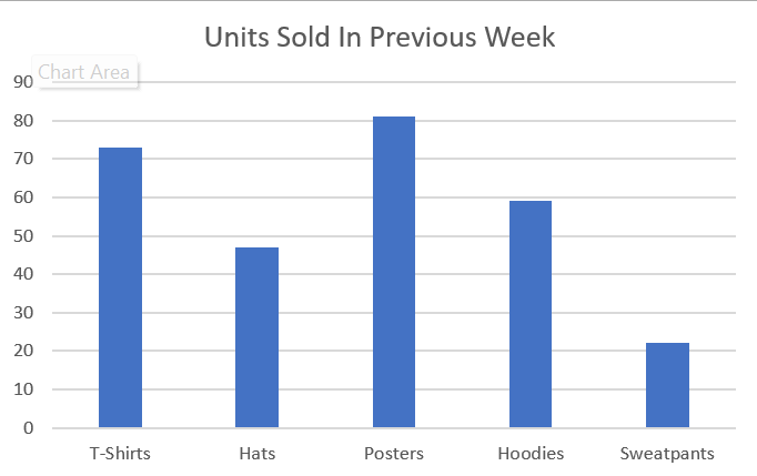
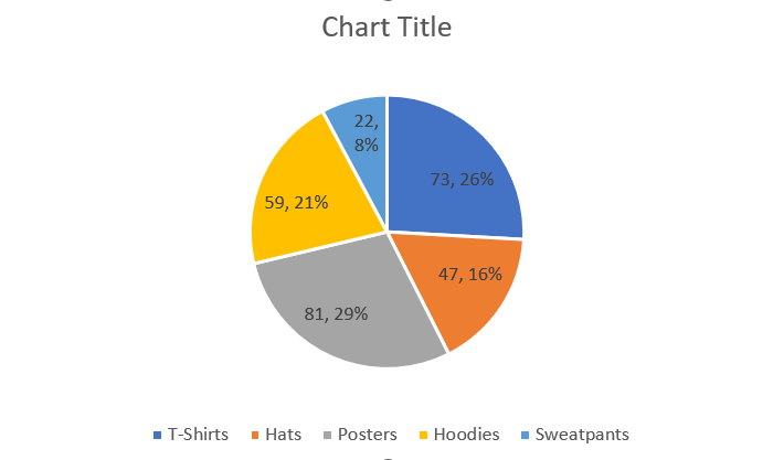
There are two commonly used types of categorical displays of data, bar graphs (or column graphs) and pie charts (or circle graphs). The data from both bar graphs and pie charts can be expressed as a frequency table or a relative frequency table.
Note that, when we use the word “units” with respect to a quantity sold in some category, we’re really counting how many are in that category. If we use, say, “T-Shirt” as a unit of measure, we can then consider it to be quantitative data.
Bar Graph
Pie Chart
Frequency Table
The information in both the bar graph and pie chart above can also be expressed as a frequency table. A frequency table is simply the count for each of the categories.
| Item
T-Shirts |
Number of units sold
73 |
| Hats | 47 |
| Posters | 81 |
| Hoodies | 59 |
| Sweatpants | 22 |
Relative Frequency Table
We can also express the frequency table as a relative frequency table. This just means that we change from the count for each category to the percentage that each count represents out of the total number of things in all the categories. Note that the percentages add up to 100% (or very close due to approximation). This must be the case for any relative frequency table.
| Item
T-Shirts |
Number of units sold
73 |
Percentage of total (expressed as a decimal) 73/282=0.2589 (to the nearest four decimal places) |
| Hats | 47 | 47/282=0.1667 (to the nearest four decimal places) |
| Posters | 81 | 81/282=0.1667 (to the nearest four decimal places) |
| Hoodies | 59 | 59/282=0.1667 (to the nearest four decimal places) |
| Sweatpants | 22 | 22/282=0.1667 (to the nearest four decimal places) |
| Total Items | 282 | 282/282=0.1667 (to the nearest four decimal places) |
Displays for Quantitative Data
As with categorical data, quantitative data has many different types of displays. Three commonly used displays of quantitative data are histograms, box-plots (also called box and whisker plots), and time series.
Histogram
A histogram uses bars similar to a bar graph. However, it’s very important to understand the difference between a histogram and a bar graph:
- A histogram represents quantitative data. A bar graph represents categorical data.
- The bars in a histogram are often referred to as “bins”
- The width of each bar (bin width) in the histogram is an interval of units. The width of a bar graph has no particular meaning.
- The order of the bars in a histogram matter. The order of the bars in a bar graph don’t matter.
Data in a histogram is organized as follows:
- Data values lie on the horizontal axis (points on the number line)
- Regular intervals (same size intervals) are marked along the horizontal axis. The width of these intervals is the bin width, and are determined in an artful fashion. What?! Art?! No formula for creating them?! Yes, we create these intervals so that there are not too many and not too few data values in each of those intervals. Why?…
- The height of each bar in the histogram represents either the frequency or relative frequency of data values in that bar. In other words the height of each bar reflects how many data values lie in the interval for that bar. The width of the bars in a histogram have to be chosen so that the shape of the outline of the heights of the bars gives us a sense of how the data distributes itself along the horizontal axis. Another way to think about this is that the shape of the distribution tells us where data is concentrated and where it’s sparse. The word “density” is used to describe a distribution of data because, a large “peak” in the outline indicates a region along the corresponding horizontal axis where data is concentrated (dense). This is a region of high or higher density than a “valley” which indicated a low or lower concentration of data (less dense) along the corresponding horizontal axis.
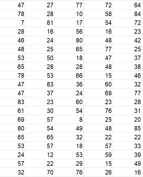
Here’s a data set of the number of t-shirts sold per event at 100 events in the past year:
Here’s it’s histogram:
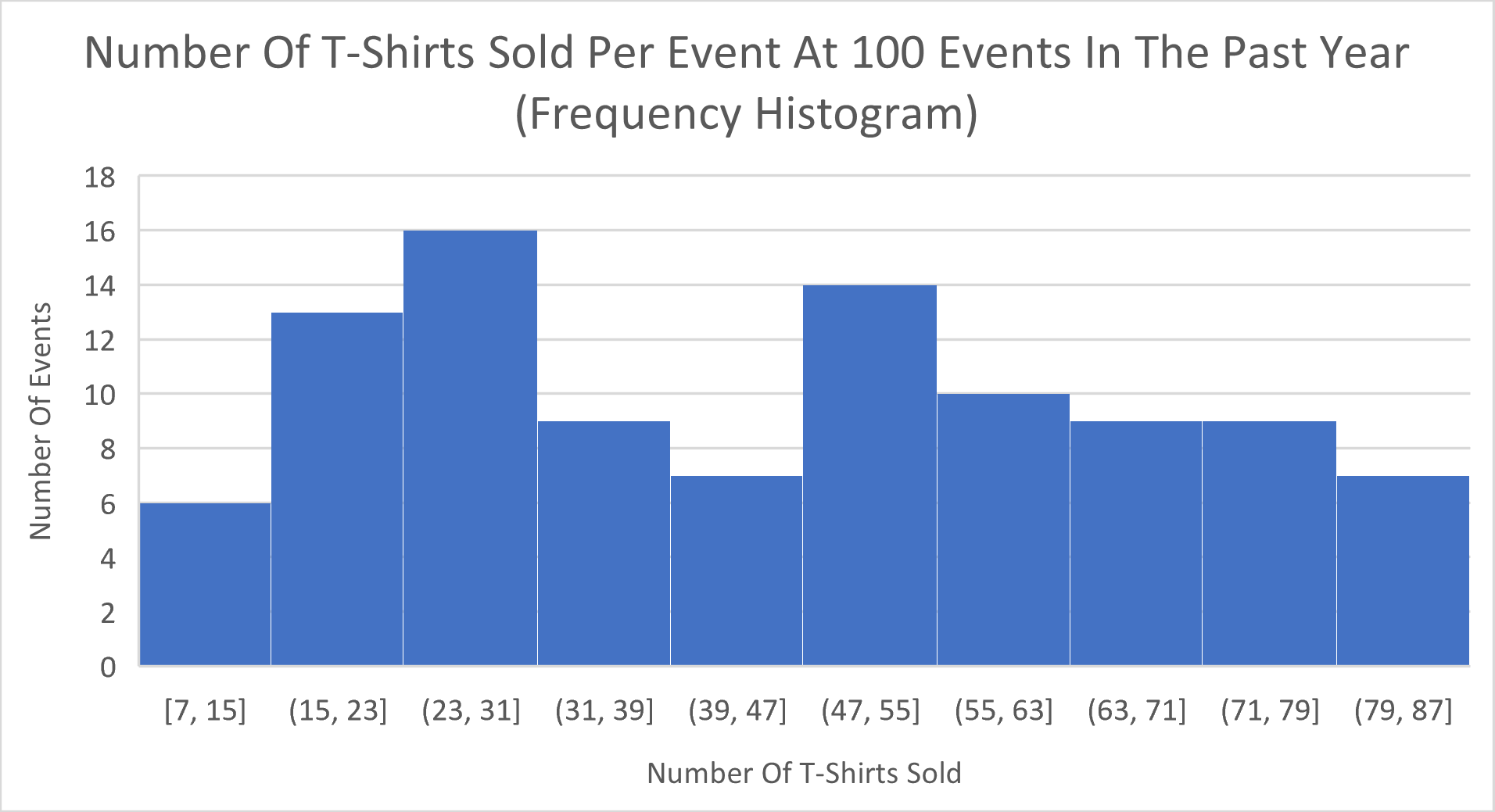
Note that the height of the bars in this histogram represent the number of data values in the respective interval (bin). That makes this a frequency histogram. Also, note that the interval width (bin width) for all bars (bins) is 8 units. This width was chosen only because it allowed the outline of the heights of the bars to show a shape. Note also that, the lowest value is 7 t-shirts sold at one event. However, the value 87 is not part of the data set. It only represents the right end of the right-most bin when we travel in steps of 8 units starting at 7 over the ten bins.
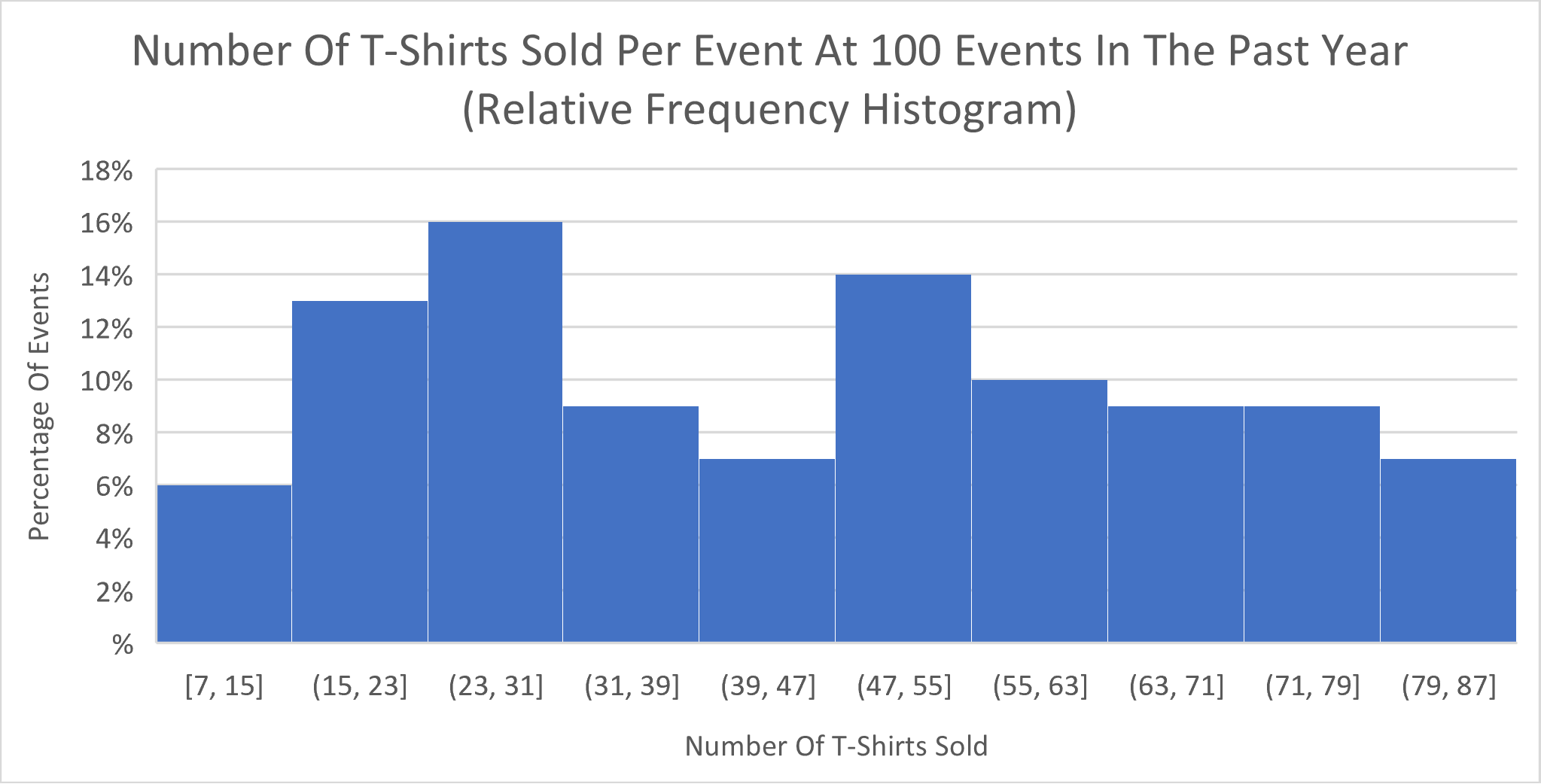
Note that, this histogram is for the same data as the previous histogram, but now the heights of the bins are percentages of the total number of data values. In this case, the total number of data values is 100, so the change from the frequency to the relative frequency for this data set is very simple. The first bin has a relative frequency of 6% because 6/100 = 6%. The second bin has a relative frequency of 13% because 13/100 = 13%. The same process applies for the rest of the bins. This implies that the total percentage for all bins is 100%.
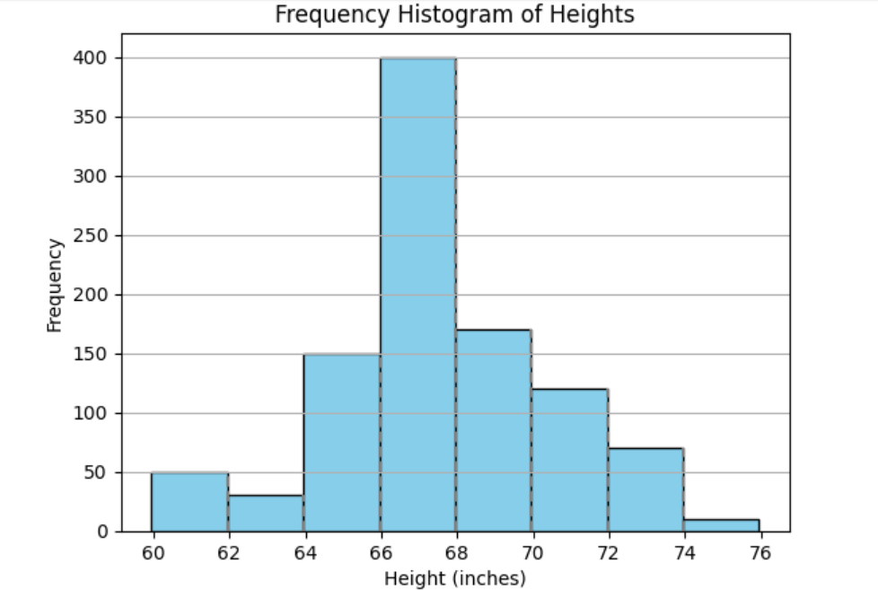
Let’s look at another histogram and practice changing from a frequency histogram to a relative frequency histogram, and then from a relative frequency histogram to a frequency histogram.
Here’s a frequency histogram. Assume that the population size is 1000, i.e., the combined frequencies of all the bins is 1000:
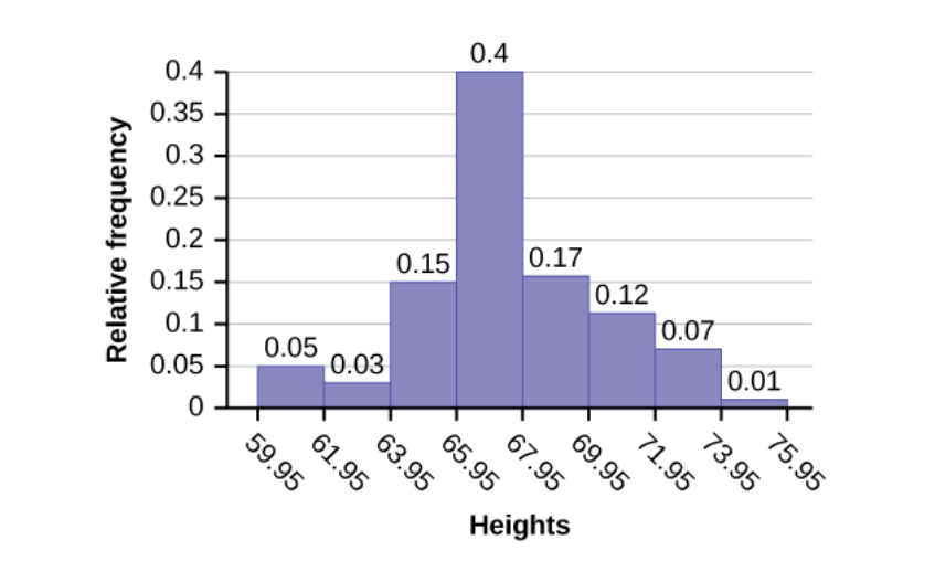
Now, here’s a relative frequency histogram:
How to create a histogram in Excel:
Link to text instructions for histogram in Excel
Link to video instructions for histogram in Excel
How to create a histogram on the TI-84:
Link to text instructions for histogram on the TI-84
Link to video instructions for histogram on the TI-84
Box-plot
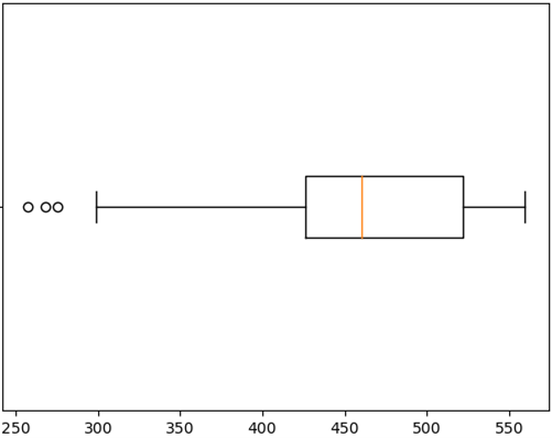
A box-plot, also called a box-and-whisker plot, takes the shape of a rectangle (the box) with lines (the whiskers) extending from two sides of the rectangle. It expresses how the data values spread themselves out along the number line (the line underneath the box-plot). The box-plot lets us know how spread out the data values are and where they’re concentrated. For the box-plot below, the rectangle contains the middle 50% of the data. The data to the left of the box is the bottom 25%, and the data to the right of the box is the top 25%. A box-plot is often oriented horizontally, but can also be oriented vertically.
Here’s a box-plot that represents the same data as the histogram for the Number Of T-Shirts Sold Per Event At 100 Events In The Past Year.
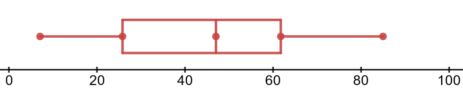
The dots on the box-plot represent, from left to right:
1) The minimum (smallest) data value. That value appears to be near 7 t-shirts.
2) The demarcation point for the 25th percentile. This is the point at which, below it lies 25% of your data values, and above it lies 75% of your data values. This point is also referred to as  , or the first quartile. This point appears to be near 25 t-shirts.
3) The median (or 50th percentile). This is the point at which half of your data values lies below it, and half of your data values lie above it. This point appears to be near 46 t-shirts.
4) The demarcation point for the 75% percentile. This is the point at which, below it lies 75% of your data values, and above it lies 25% of your data values. This point is also referred to as  , or the third quartile. This point appears to be near 62 t-shirts.
5) The maximum (largest) data value. This point appears to be near 85.
6) The distance from to is called the Inter-Quartile Range, or IQR. It’s a measure of how spread out the data is. So, for this box-plot, the IQR is 62-25=37 t-shirts. We measure spread using the same units as the data values.
The values for items 1 through 5 are often referred to as a 5-Number Summary
Note that the median for a box-plot isn’t always in the center of the box. When the median is closer to the left side of the box, the bottom 50% of the data is concentrated in a smaller interval, and the data to the right of such a median is more spread out. We’ll discuss this more in the next section.
It’s also important to note that the values for , the median, and might or might not be data values. They are points on the number line which serve to separate the data values into certain regions.
Outliers
There’s one more important thing we need to know about box-plots and data in general. Outliers are data values which are far from most of the other data values. What does it mean to be far from the other data values? It can mean several things:
- The data value is simply an unusual value for the population from which the sample was taken, but it belongs with the other data values.
- The data value is associated with some condition which makes it different from the population which the sample was drawn from. An example of this could be average daily wind speed for some location which had experienced a hurricane on one of the days in the year’s worth of average daily wind speeds.
- The data value is a result of measurement or input error.
We should always note when there are any outliers in the data so that the data set is typical of the population from which it was drawn.
In a box-plot, an outlier is a data value which is either more than 1.5 IQR below or more than 1.5 IQR above . We call the cutoff points for outliers “fences”. So, any data value that is below the lower fence is an outlier, and any data value which is above the upper fence is also an outlier. The fences are not usually shown in a box-plot, but we can imagine where they are by using the IQR (the length of the box) and measuring 1.5 times that length below and above . Remember that the left end of the box represents , and the right end of the box represents . It’s important to note that the end of the whiskers are usually not the fences. When no outliers are marked in the box-plot, then the end of whiskers are the minimum and maximum values. When outliers are present, the end of the whisker(s) are just the least or greatest data value which lies within the fences.
In a box-plot, we use a dot (or small circles) to represent data values which are outliers. The three little circles to the left of the whisker in the box-plot below are outliers. Each one of these data values are more than 1.5 IQR below . The end of the left whisker is the smallest data value which lies above the fence. The end of the right whisker is the maximum data value because there are no high-end outliers for the data which this box-plot represents.
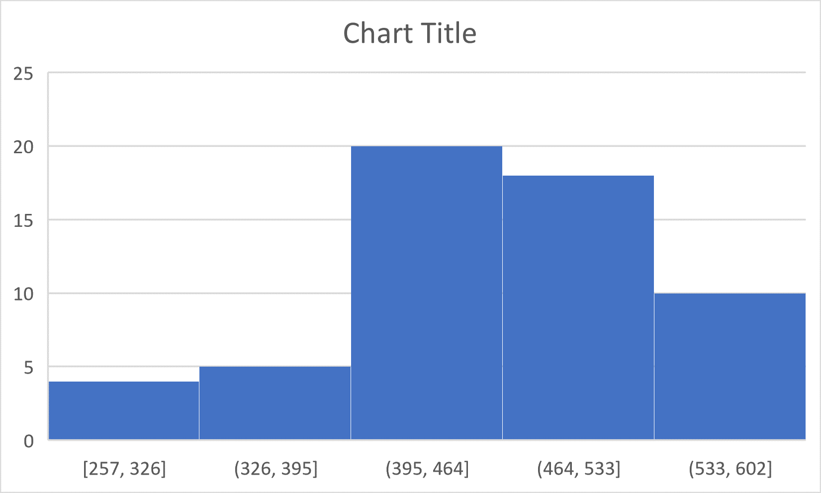
As a comparison, below is the histogram of the same data set. Notice how the outliers aren’t apparent in the histogram.
How to create a box-plot in Excel:
Link to text instructions for box-plot in Excel
Link to video instructions for box-plot in Excel
How to create a box-plot on the TI-84
Link to text instructions for box-plot on the TI-84
Link to video instructions for box-plot on the TI-84
Time Series
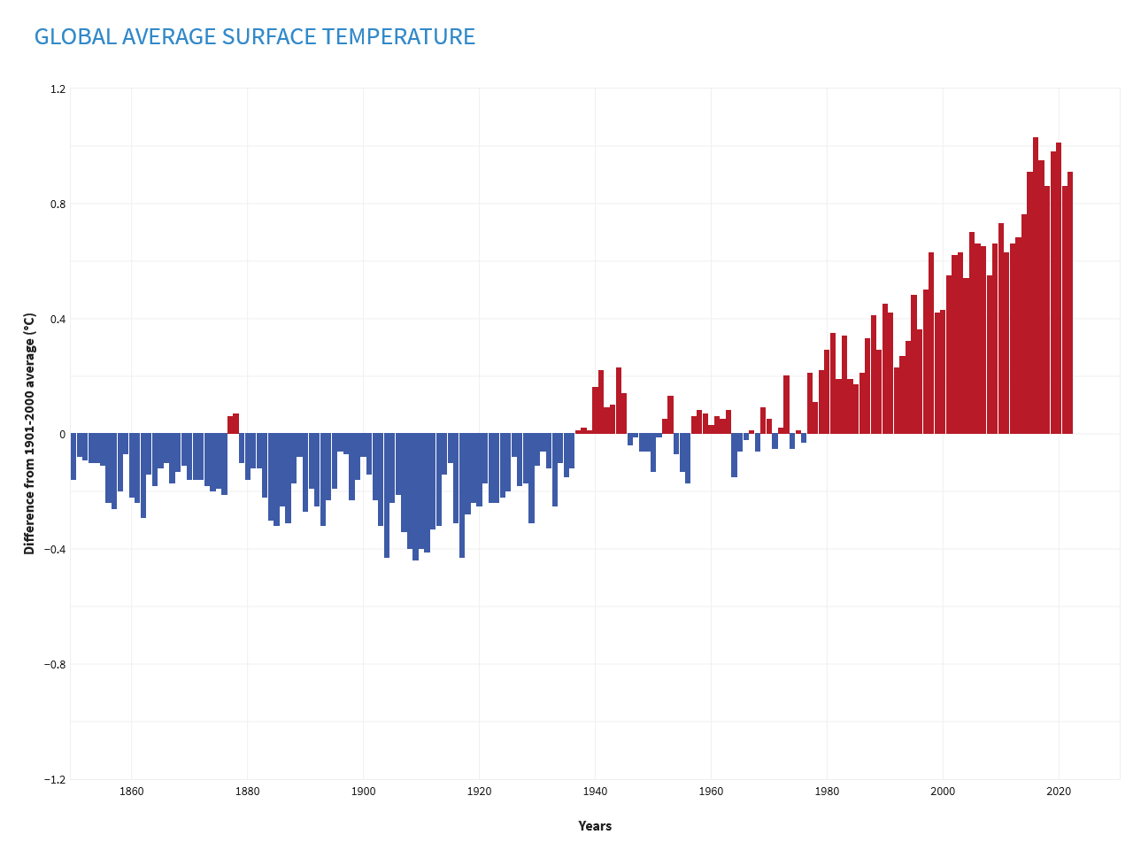
A time series is a sequence of points that can rise and fall. The points represent some particular measurement like temperature or money or any other quantitative data. The horizontal distance between points is some unit of time. Time series can have each point connected by a line segment, or each point can be at the top of a bar.
Here’s an example of a time series where each point is the top of each little bar, and each bar represents the global average surface temperature for that year as some number of degrees Celsius above the 20th-century average of 13.9 °C:
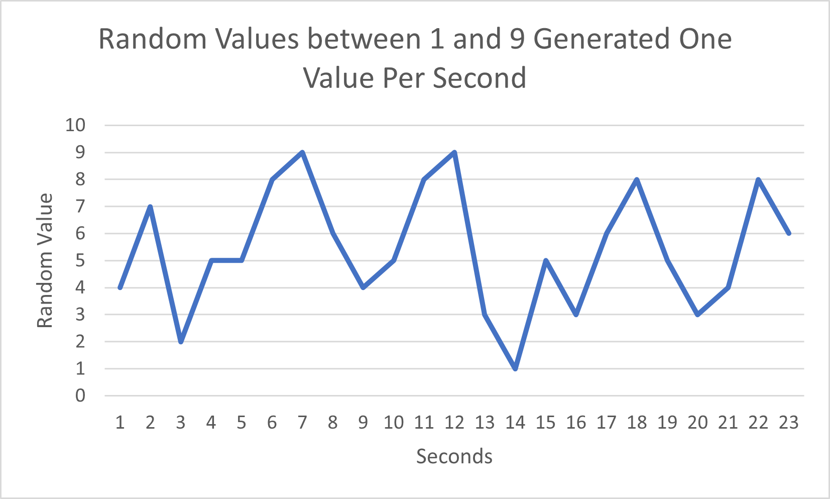
Here’s an example of a time series where each point is connected by a line segment:
Other Ways To Display Data
There are many ways to display both categorical and quantitative data. For this course, we will focus on bar-graphs, histograms, and box-plots. Here’s a link which you can look at (but won’t get tested on) other displays of data:
Link to Wikipedia entry for data visualization techniques
ChatGPT
4.4 – What Does The Data Tell Us?
Summary Data From Tables and Visual Displays
Data can be summarized using tables and visual displays like box-plots, and the shape of a histogram can give us information about the data. This section gives us an introduction to these types of summary data and visual displays.
So, what can we expect if we’d like to know how long it might take for someone at our phone company to answer our call while we wait on hold? The automated system will sometimes tell us approximately how long it will take for someone to answer our call. But how does it know how long it will take?
Let’s suppose there’s only one customer service person working, and that there are 7 people ahead of you in the cue waiting to speak with that customer service person. How might we estimate the time it will take for someone to help us?
Now, let’s suppose that the following table is a list of the amount of time each person in the cue spent with the customer service representative:
| People | Time spent with customer service in minutes |
| Person 1 | 6 |
| Person 2 | 4 |
| Person 3 | 7 |
| Person 4 | 15 |
| Person 5 | 27 |
| Person 6 | 14 |
| Person 7 | 5 |
So, the actual time that you waited was 78 minutes. If you had known that you would have spent that much time waiting, would you have waited?
If you had the list of times in the table to begin with, you could make a decision whether to wait or call back another time. But what if we could get a long list of individual times from the same day and time from the previous week? Might that help us make a decision?
The point here is that we can use the data from a recent previous time to help us make a decision now. However, we must take note of whether the data is representative of the time at which we call the phone company. Remember, things can change, and some call times have different patterns than others.
Population and Sample
A population is simply the group of people or things that we are interested in examining. A sample is a subset of the population.
We can’t always examine every person or thing in the population because the population might be very large. So, we take a sample from that population. If we examine every person or thing in the population, then we have a census.
Example of a Sample: We select 30 people in some city, and ask how they will vote for some proposition on the city ballot. The 30 people are a sample. The type of data we collect in this case is categorical.
Example of a Sample: We select 30 people in some city and we ask them about their commute time (in minutes) to work on the past Monday. The 30 people are a sample. The type of data we collect in this case is quantitative.
Example of a Census: Every four years in the U.S., a census of the population is done. The questions range from number of people in each household (quantitative) and the number of people in different age brackets (categorical) to race (categorical) to relations within a household (categorical).
When we look for data that can help us answer a question, the data must be selected so that it is representative of the population we’re interested in. If we want to estimate how long it will take for the phone company to answer our call, then the data that we collect about individual times spent with customer service must reflect the typical customers of that phone company. We should also consider the geographical location of the customers, because different locations often have different issues.
Measures of Center and Typical Values: Mean, Median, and Mode
We need a way to express the typical data value in a set of data values so that we can make decisions given that the data values vary. So, can we find one value which, somehow, represents all of those data values? There are many ways to do this, but the most commonly used measures for this are the mean, the median, and the mode. The mean and the median are used for quantitative data. The mode can be used for quantitative and categorical data.
Mean
You might have already known that if we have an average time for a list of various times in a table like the one above, then we can know approximately how long we will wait given some number of people in the cue. So, in the example above, the average time spent with customer service for the seven people in front of us in the cue is obtained by adding each value and dividing by the number of data values:
6+4+7+15+27+14+5 = 78
78/7 = 11.1428714 (approximately)
Notice that, if we multiply the average time (11.1428714) by the number of people (7), we get 78. This makes sense because, we’re breaking up the entire time of 78 minutes into 7 equal parts.
Another word for average is “mean“. If we let  be the ith x value in a set of values, and if we let
  be the mean of the x values in the set of values, then a math formula for the mean is given as follows:

This formula just says that if we add up each of the data values and divide by the number of data values n, we obtain the mean. We will note that, for this formula, each of the data values has equal weight. This means that each data value has the same chance of occurring or counts the same as any other. Later, we’ll see a more general formula for the mean which takes into account the weight of each data value.
We use two different letters to represent the mean of the population and the mean of a sample. We use the Greek letter μ to represent the mean of a population, and we use to represent the mean of a sample. The mean of the population, and the mean of a sample both use the same formula given above.
Also, the mean of a data set need not be a data value in the data set.
Note: Do not use the mean for ordinal data!
As mentioned in the section about ordinal data, we must not treat ordinal data (data like ratings of 1 to 5 for some product or service) as quantitative data. This implies that we should not take averages of ordinal data because there’s no underlying unit of measure for ordinal data.
Beware of any study or experiment which uses the mean for ordinal data!
Unfortunately, and all too often, people treat ordinal data as if it were quantitative data. Doing so produces nonsense because ordinal data is subjective (differs from person to person). So, if a survey asks about your experience for some product or service, you might feel that a good experience is a “4”, and another person may feel that a good experience is a “3”, and another person…I think you get the idea. Also, and reasoning similarly, there’s no way to take a meaningful sum or difference of two ordinal scores. All we can do with ordinal data is get a frequency count (or relative frequency) for each of the response levels. To be honest, there are some sophisticated methods of teasing out some useful information from ordinal data (also called Likert data). However, even when we use those techniques, the information that we get from ordinal data can be very limited.
How to calculate the mean on Excel
Link to text instructions for creating the mean in Excel (Please see the Excel help in the Websites module on Canvas)
Link to video instructions for creating the mean in Excel
How to calculate the mean on the TI-84
Link to text instructions for creating the mean on the TI-84 (Please see the “Using the TI-83, 83+, 84, 84+ Calculator” in section 2.5 of the OpenStax text)
Link to video instructions for creating the mean on the TI-84
Median
As we saw in the box-plot, the median is the value which separates the data set into two equal halves. Below it is 50% of the data, and above it is 50% of the data. To obtain the median from a data set, we first order the data values from smallest to largest, then we choose the middle value. If we have an even number of data values, then we take the average of the two middle values. We note that, when there’s an odd number of data values, using the middle value will separate the data set into two equal halves, but each half is not exactly 50% of all the data values. This is not usually a problem unless we need to have a data set which has exactly 50% of the data above the median and 50% of the data below the median.
Also, when we have an odd number of data values in the data set, the median will be a data value in that data set. When we have an even number of data values in the data set, the median will not be a data value in that data set.
As with the mean, do not use the median for ordinal data!
How to calculate the median in Excel
Link to text instructions for creating the median in Excel (Please see the Excel help in the Websites module on Canvas)
Link to video instructions for creating the median in Excel
How to calculate the median on the TI-84
Link to text instructions for creating the median on the TI-84 (Please see the “Using the TI-83, 83+, 84, 84+ Calculator” in section 2.5 of the OpenStax text)
Link to video instructions for creating the median on the TI-84
Mode
The mode is the value in the data set which occurs most often. When there’s a tie for which data value occurs most often, then we can have multiple modes. Also, we can consider second place modes or third place modes for data values which are second most frequent or third most frequent.
Things to remember about modes:
- In a histogram, the midpoint of the tallest bin is considered the mode, even though it’s possible that the mode of the data set is in another bin.
- Multiple modes might or might not indicate groups within the data which are in some way different from each other. The more pronounced the peaks are, the more likely that it indicates separate groups within the data. When the peaks are less pronounced, they might just be due to chance.
- Modes indicate where the data is concentrated.
- Modes can be used for categorical and ordinal data.
In the relative frequency histogram below, we see a mode for the bin 65.95 inches to 67.95 inches. So, we take the midpoint of that bin to be the mode of the histogram. The midpoint of that bin is (65.95+67.95)/2 = 66.95. The relative frequency of that bin is 0.4 or 40%. This means that 40% of all the data which makes up this histogram lies in that bin. We don’t usually think of the left-most bin (59.95 to 61.95) as a likely candidate for a mode just because it forms its own little peak, especially because only 5% of the data exists in that bin. It’s very important to know that, when we sample data from a population, the shape of the histogram will vary a bit from sample to sample. We don’t expect big differences in the shape of the histogram each time we sample from a population, just small differences. Occasionally, sampling can give us a shape that appears different than the histogram of the data from which we sampled it.
How to calculate the mode on Excel
Link to text instructions for finding the mode in Excel (Please use the Excel help in the Websites module on Canvas)
Link to video instructions for finding the mode in Excel
How to calculate the mode using the TI-84
Link to text instructions for finding the mode on the TI-84 (Please use the Try It example 2.34 in section 2.7 of the OpenStax text)
Link to video instructions for finding the mode on the TI-84
Measures of Spread: Standard Deviation and IQR
Since data varies, we would like to know by how much it varies because this can help us make decisions. If the data values are all close to each other, we can more easily decide whether the time that it will take to speak with customer service is likely to be a time interval which we can tolerate. If the data values are very spread out, it makes it more difficult to know what we can expect. A mean or median of a data set can give us some idea of how long we might wait given many attempts at calling the service center at our phone company, but each time we call, we’re faced with the possibility of waiting longer than the mean or the median, or waiting less than the mean or the median.
Standard Deviation
The most often used measure of spread for data is the standard deviation. When we use the standard deviation as a measure of spread, we use the mean as the measure of center or typical value. In fact, the standard deviation can be thought of as the typical distance that the data values are from their mean.
Note: The standard deviation is always positive and has the same units as the data.
The formula for the standard deviation adds up the squared differences that each data value is from the mean, then it divides that result by either the number of data values (for the population) or the number of data value minus one (for a sample), and then it takes the square root of the result. The letter s is used to represent the standard deviation. Here are the formulas:
Standard deviation for the population
 ,
,
where 
Standard deviation for the sample

where 
If we square the standard deviation, we get the variance.
Variance for the population

Variance for a sample

The variance has a special use which we will see later in this course.
We won’t need to calculate the standard deviation by hand. We will use technology.
How to calculate the standard deviation on Excel
Link to text instructions for calculating the standard deviation on Excel (Please use the Excel help in the Websites module on Canvas)
Link to video instruction for calculating the standard deviation on the Excel
(Note: The video uses STDV.S. This is the standard deviation of a sample. If we want the standard deviation of the population, we use STDV.P)
How to calculate the standard deviation on the TI-84
Link to text instructions for calculating the standard deviation on the TI-84 (Please use the Try It example 2.34 in section 2.7 of the OpenStax text)
Link to video instructions for calculating the standard deviation on the TI-84
IQR (Inter-Quartile Range)
The IQR was introduced earlier when we looked at box-plots. Similarly to the standard deviation, it’s a measure of how spread out the data is. However, the IQR is not usually the same distance as one standard deviation. When we use the IQR for the measure of spread, we use the median as the measure of center or typical value.
Parameters and Statistics
A parameter is a value that represents a population. A statistic is a value that represents a sample.
Mean of population – We use the Greek letter μ (pronounced like the word “you” with the letter m in front of it) to represent the mean of the population.
Mean of a sample – We use the letter to represent the mean of a sample.
Standard deviation of a population – We use the Greek letter σ (pronounced “sigma”) to represent the standard deviation of a population.
Standard deviation of a sample – We use the letter s to represent the standard deviation of a sample.
Shape Of A Distribution For Histogram and Box-Plot
The shape of a histogram and the shape of the box-plot say a lot about the data. The shape indicates how the data distributes itself over the range of its values. It should be the first thing that you look at if it’s available. If it’s not immediately available, then creating a display from the data set is advisable when possible.
Here are the five main distribution shapes:
1) Uniform – Histogram is mostly flat, but it can have bins that are taller or shorter.
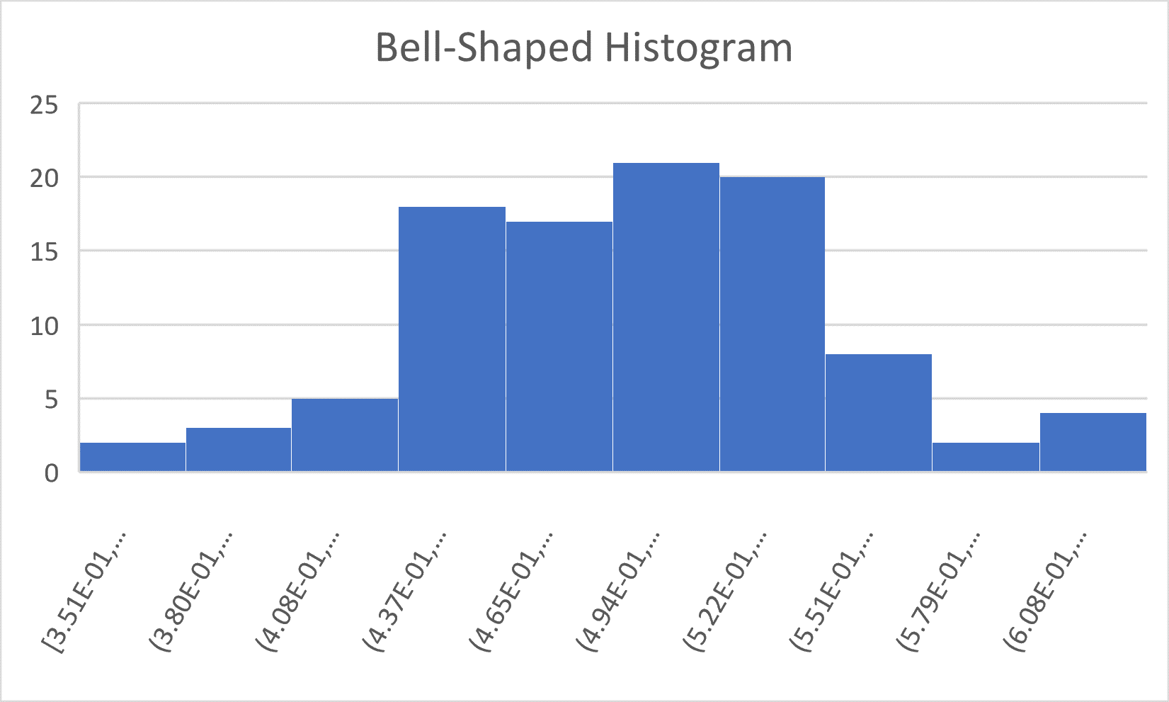
2) Bell-shaped – (unimodal and mostly symmetric) – A histogram with a, mostly, bell shaped outline is one of the most common shapes in statistics. This shape is very important for the math of statistics.
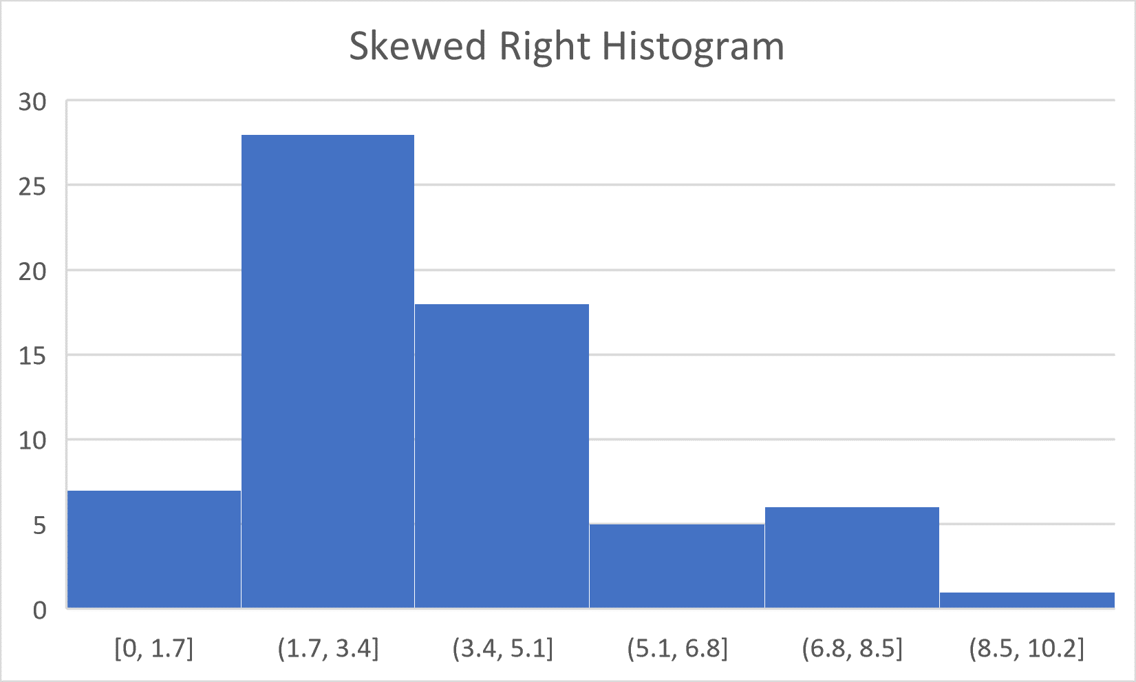
3) Skewed Right – A histogram which has a longer taper to the right is considered to be skewed to the right. The mode of this frequency histogram is the midpoint of the second bin (1.7+3.4)/2 = 2.55. The data is concentrated in that bin the and the one to its right, and it tapers to the right.
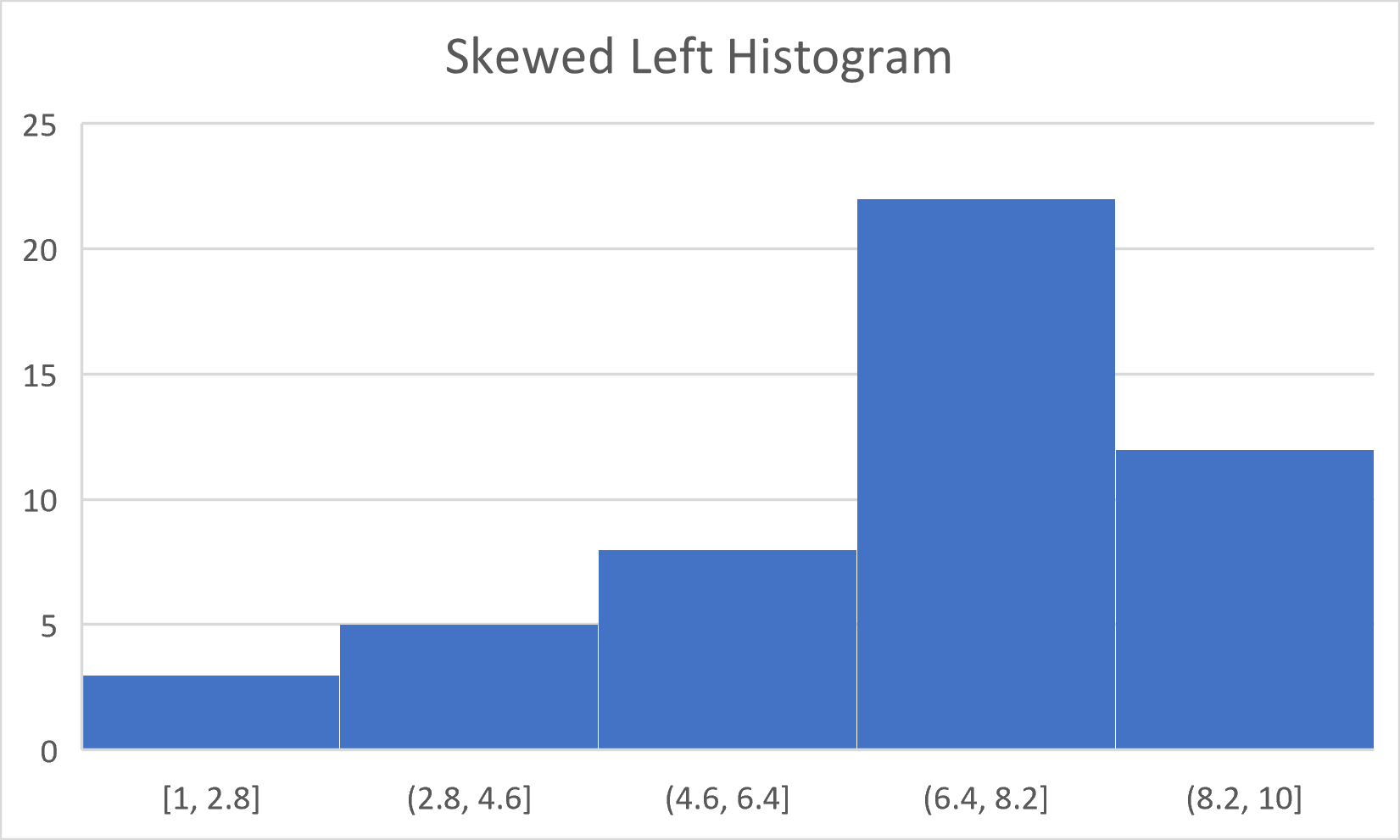
4) Skewed Left – A histogram which has a longer taper to the left is considered to be skewed left.
Remember that, in a histogram, the peaks are where data is concentrated. For the following histogram of the Number Of T-Shirts Sold Per Event At 100 Events In The Past Year, we see that there are roughly two peaks. One peak is at the third bin (23 to 31 t-shirts sold), and the other peak is at the sixth bin (47 to 55 t-shirts sold).
So, what might it mean that we have two peaks for this data?
Before we give an answer to the previous exercise, let’s think about the shape of a histogram for a 10 kilometer run. Can you think about what the distribution of the finishing times for the race might look like?
What might the distribution of incomes in Seattle WA look like?
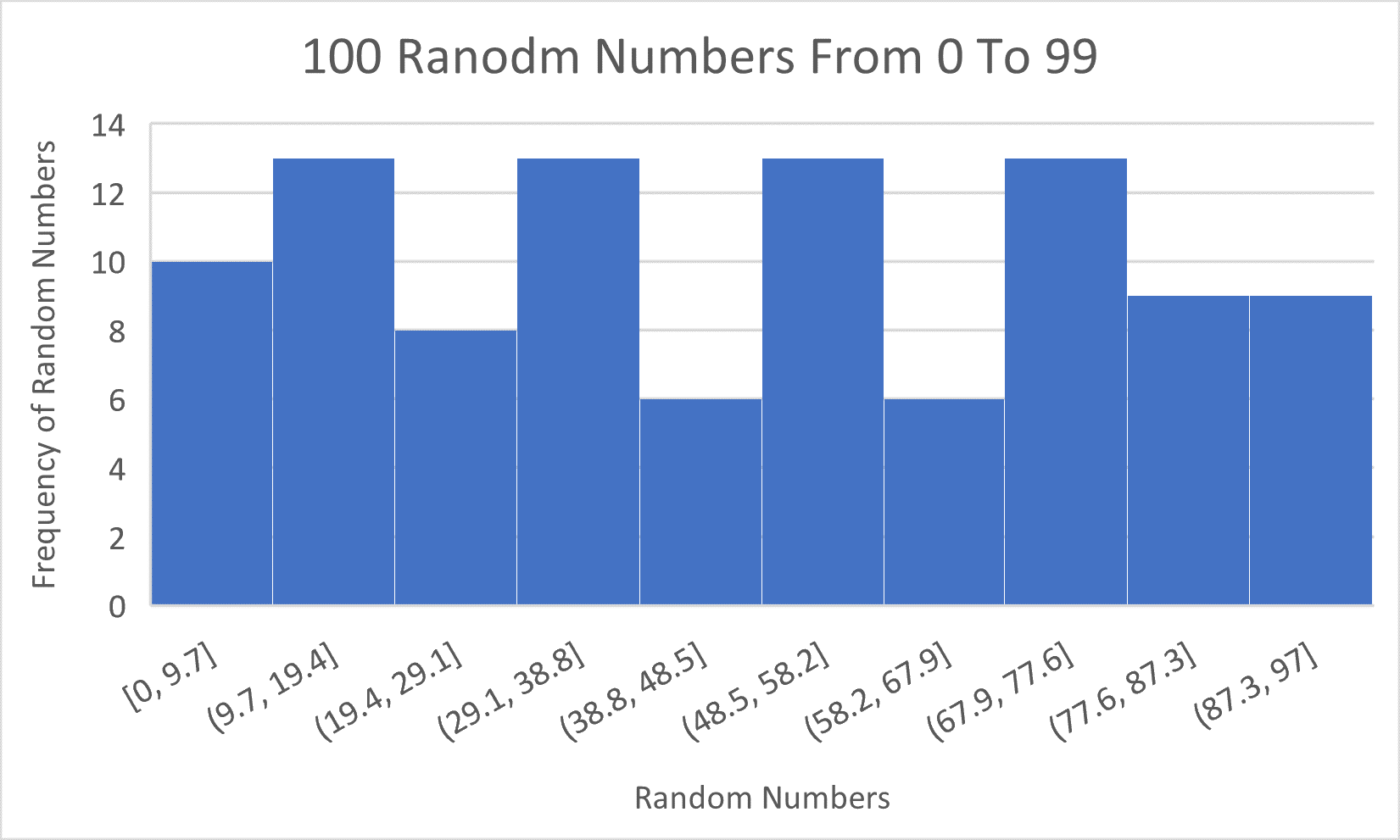
What might the distribution of random numbers between 0 and 100 look like?
Now, getting back to the T-Shirt histogram, are the two peaks (modes) meaningful? Could they be a result of smaller or larger events? Or might these peaks (modes) be due to chance?
It turns out, that the histogram of T-Shirts was generated by random numbers which have an underlying uniform distribution. So, why does the histogram appear to be bimodal? Because when we sample from a population with any distribution, the resulting histogram of the sampled data will usually resemble the histogram of the population from which we drew our sample, but it can vary due to chance.
4.5 – A Random Sample Gives Us A Representative Sample
We get a representative sample by selecting randomly. Why does a random selection give us a sample which is representative of the population from which we draw it? Because it doesn’t favor any one thing that might distort the sample. It selects without bias.
Random selection is usually implemented using a random number generator. Here’s a link to the website Random.org. Suppose we have 100 people or things in our population and we’d like to randomly select 10 people or things. To use the random number generator to make a random selection, we first label each of the people or things in the population with a unique number 1 through 100. Then we go to the random number generator and have it give us ten numbers whose value is any number, 1 through 100. We then select the people or things in our population which have those randomly generated numbers.
Now try this by going to Random.org and in the “Numbers” sections choose “Integer Generator”. Then input the following into the fields in Part 1: The Integers:
Generate 10 random integers.
Each integer should have a value between 1 and 100.
Format in 1 column.
Your result is an example of the ten random numbers referred to in the previous paragraph. Each time you create a random sample, it will almost always be different from any other random sample. You can do this several times to see what happens.
When we create a random sample in the manner described above, we have created a special type of random sample called a simple random sample. This type of random sample allows for all subsets of the population which are of the same size to have the same chance of being selected. A simple random sample is the gold-standard of samples. It’s the method that has the smallest chance of introducing bias into the sample. The less bias that a sample has, the more representative it is of the population.
However, we can’t always create a simple random sample. Imagine trying to create a simple random sample of 1000 people spread across the U.S.. Trying to assign a number to each person in the U.S. isn’t possible, let alone getting them to participate in whatever survey one might do. For smaller populations such as Renton WA, if we’re interested in how people in Renton WA might vote on a particular issue, we can use list of registered voters in Renton WA, number them, and then use a random number generator to select the sample. When we use a list to randomly select from, we call the list a sample frame. A sample frame should be representative of the population which one is trying to estimate.
Other Sampling Methods
As mentioned above, we can’t always get a simple random sample. So, we use other methods to get a reasonably representative sample. Here are three other methods which are commonly used.
Cluster Sampling
To get a cluster sample, we find a subset of the population which we believe to be representative of that population, and then we take a random sample from that subset.
Example: A residential block in Renton WA is chosen to see how they will vote on some issue on the upcoming ballot. The block contains both homes and rentals in about the same proportion as all of Renton WA, the income level on that block is typical of Renton WA, and the block is representative of the racial, ethnic, and national status of Renton WA. Notice how we chose this block based on how similar it is to all of Renton WA. This helps to make the sample representative of the population.
Systematic Sampling
We get a systematic sample by selecting every nthperson or thing that is in some order
Example: We select every 7th person in line for movie to ask them about their preference for toothpaste. We select the first person by randomly choosing a number between 1 and 7, say 4, and then start with the 4th person and choose every 7th person from that 4th person. Notice that we use random selection within methods that are not themselves completely random. We do this to obtain a representative sample.
Stratified Sampling
We use stratified samples to ensure that one group doesn’t dominate the sample simply by an unlucky random selection. We do this when we have reason to believe that one group might have a different opinion or status than the other group. We obtain a stratified sample by randomly selecting from one group and then randomly selecting from another group. However, the number of random selections from each group depends on the ratio of their occurrence in the population that we’re trying to estimate.
Example: A city wants to decide if they should build a new park. However, the funding for the park will come from property tax. If 65% of the city’s residents are homeowners, and 35% of the city’s resident’s are renters, and if we want to have a sample size of 250 city residents, then we randomly sample 0.65×250 = 163 property owners and 0.35×250 = 88 renters. This way we get a representative sample with respect to a factor that will likely bear on the issue that we’re examining. Had the funding for building the new park not been based on property tax, but instead based on funds obtained from the state for local improvements, we wouldn’t need to stratify our sample because property owners and renters would not likely have any difference in how they might vote on such a measure.
4.6 – What Would We Like To Know? What Type Of Questions Can We Ask?
It’s very easy to ask a question that seems very simple, but often requires much more analysis that one might think. We will continue to use the techniques that we’ve developed in this course to ask more focused questions that help us answer bigger questions.
5-Number Summary - Summary data consisting of the minimum data value, the first quartile (25th percentile known as Q1), the median (50th percentile also known as the second quartile), the third quartile (75th percentile know as Q3), and the maximum data value.
