5 Chapter 5 – What’s The Probability?
5.1 – Origins and Foundations
The probability of something occurring is the chance that it happens described by a number between 0 and 1 (including the possibility of 0 or 1). You’ve might have asked about the chances of something happening and received a response of 50%. This means that the chance that it happens is the same as the chance that it doesn’t happen. What would you think the chance of a light being on and off at the same time is? If you answered 0, you’re starting to understand what probability is. If the probability of something happening is 0, then it doesn’t happen. If the probability of something is 1, then it must happen.
Probability theory is the foundation of statistics. It’s a beautiful and deep subject in mathematics, but the basic ideas are not difficult to grasp. So, we will work on getting a firm grip on the fundamental concepts, and then we’ll use those concepts in a way which, hopefully, won’t overwhelm the reader with details.
Much of the early history of probability theory comes from games of chance. Games involving dice, cards, spinners, and other devices that create the element of chance and make the game exciting. People have bet money and possessions on these games since the games were first developed. The lure of winning a large sum of money or goods on the roll of two dice is hard to resist, and it’s easy to lose more money than one wins. So, people have studied the outcomes of repeatedly rolling the dice or drawing cards and come to the conclusion that certain dice rolls and certain card draws are more or less likely. These observations are the beginning of probability theory and statistics.
Some games are designed so that the best an individual can do when playing the game is to lose as little as possible. Each casino in Las Vegas NV makes about $21.5 million per day! How do they manage to make that much money from the people who patronize those casinos? They don’t charge an entrance fee, and they’re not making too much money on anything other than gambling. So, one might think that no one would go to a casino if they were going to lose a lot of money. Yet the patrons lose more money than they win. How does that happen?
There are two factors that make casinos the money machines that they are: 1) The chances that the casino (also called “the house”) wins is, overall, only slightly greater than 50% of the time, and 2) The number of people who go to the casino over a year’s time is very large. Since the chances of the casino winning is a bit more than 50% of the time, the chance of the patron winning is a bit less than 50% of the time. However, if many patrons are betting, then many will win. So, it’s virtually impossible for the patron to detect how often the casino wins compared to how often the patrons are winning, especially with the deleterious effects of alcoholic beverages.
From these games of chance, humans adapted and expanded the concepts of probability to business and science. We will now look at the underlying principles of probability.
5.2 – Probability Space, Outcomes, and Events (Venn Diagrams)
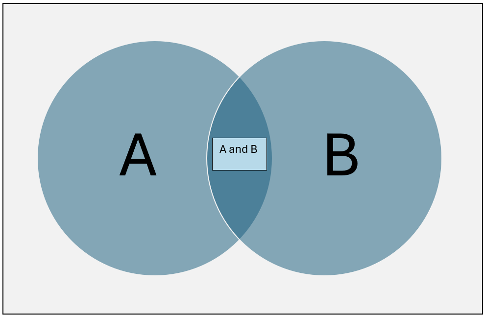
The easiest way to understand how probability works, and to be able to apply it when you need it, is to know that events like rain or accidents or sunny days or red lights at an intersection can be measured. How can they be measured? We can think about an event as some part of a bigger picture where this bigger picture is all possible outcomes that relate to the event or events. Then, we can think of any event as being some part of the bigger picture. So, we measure each event by giving it a percentage (or a decimal) which corresponds to how likely it is to occur with respect to the bigger picture. This percentage or decimal is the probability measure (or just probability) of the event. The bigger picture is sometimes called the universe or probability space. We let the universe have a percentage of 100% so that everything in the universe (probability space) adds up to 100%. This means that the probability measure of the probability space is 100% or 1.
Here’s a picture where the circles represent events (we leave the events to your imagination), and the rectangle represents all possible outcomes relating to the events, i.e., the universe or probability space.
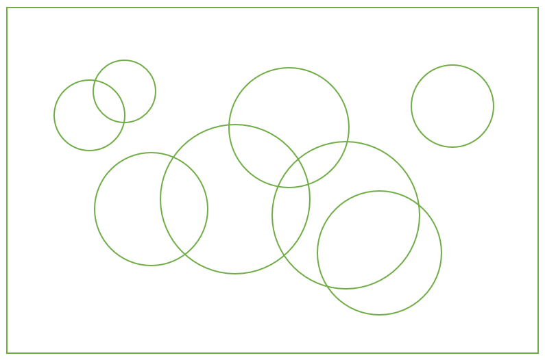
The size of the circles don’t necessarily represent how likely the event is. In fact, when we draw these types of pictures, the size of the circles usually don’t represent how likely they are. The circles are just there to let us know that we’re referring to an event in the universe of possible outcomes represented by the rectangle.
This type of representation of a probability space is called a Venn Diagram after John Venn introduced them in the 1880’s.
We can think of outcomes in a probability space as the atoms, and the events as molecules. In the same way that molecules are made of atoms, events are made of outcomes. For example, if we toss a single six-sided die the possible outcomes are 1, 2, 3, 4, 5, and 6. If we toss two six-sided die, the event that we roll a 7 is made from the outcomes of two dice that we can label green and red. The table below gives all the outcomes of these two dice which make up the event that we roll a 7.
| Green | Red |
| 1 | 6 |
| 2 | 5 |
| 3 | 4 |
| 4 | 3 |
| 5 | 2 |
| 6 | 1 |
So, there are 6 outcomes that make up the event that we roll a 7.
Now, let’s think of the circles as the outcomes of dice rolls:
When it comes to rolling a pair of dice, each outcome is equally likely. When outcomes are equally likely, then the probability of those outcomes are said to be equal. For some probability spaces, not all outcomes have the same probability. For example, if the probability space consists of the phases of a traffic light (green, yellow, and red), then each color of the traffic light is an outcome in that probability space. However, as we’ve probably experienced, the probability of a green light when we approach an intersection is not the same as the probability of a yellow light because a yellow light lasts only a very short amount of time compared to a green light.
So, when we count outcomes and use them to get the probability of some event which is made up from some of the outcomes, we must be careful to think about whether the outcomes are equally probable. If the outcomes are equally probable, then we can calculate the probability of an event by counting the number of outcomes that lead to the event, and then dividing that number by all possible outcomes in the probability space.
Example: The probability of rolling an 8 using a pair of dice can be calculated by first counting the number of outcomes that give us a total of 8, and then dividing that number by all possible outcomes. So, how many outcomes give us a total of 8? Consider two dice, one which is green, and the other which is red:
| Green | Red |
| 2 | 6 |
| 3 | 5 |
| 4 | 4 |
| 5 | 3 |
| 6 | 2 |
So, there are 5 outcomes that give us a total of 8.
Next, how many possible outcomes are there in the probability space for rolling a pair of six-sided dice? In the table below, we see that there are 36 possible outcomes for rolling a pair of six-sided dice:
| Green | Red |
| 1 | 1 |
| 1 | 2 |
| 1 | 3 |
| 1 | 4 |
| 1 | 5 |
| 1 | 6 |
| 2 | 1 |
| 2 | 2 |
| 2 | 3 |
| 2 | 4 |
| 2 | 5 |
| 2 | 6 |
| 3 | 1 |
| 3 | 2 |
| 3 | 3 |
| 3 | 4 |
| 3 | 5 |
| 3 | 6 |
| 4 | 1 |
| 4 | 2 |
| 4 | 3 |
| 4 | 4 |
| 4 | 5 |
| 4 | 6 |
| 5 | 1 |
| 5 | 2 |
| 5 | 3 |
| 5 | 4 |
| 5 | 5 |
| 5 | 6 |
| 6 | 1 |
| 6 | 2 |
| 6 | 3 |
| 6 | 4 |
| 6 | 5 |
| 6 | 6 |
Each of these possible outcomes are equally likely, and together these possible outcomes make up the entire probability space. So, to get the probability of rolling an 8 we can form the fraction  . This fraction represents the probability of rolling a total of 8 using a pair of six-sided dice.
Probabilities using histograms
Venn Diagrams are not the only way that we can express probabilities. Let’s look at how probability can be expressed using histograms. Here’s a histogram we saw in chapter 4. We will assume that the data that makes up this histogram represents the entire population and not just a sample. So, we can assume that the histogram accounts for the entire probability space of heights.
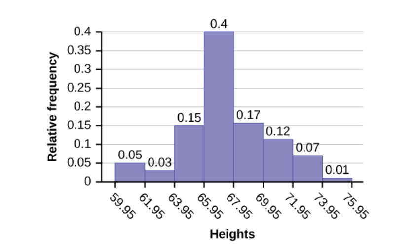
The histogram above is a relative frequency histogram. A relative frequency histogram allows us to easily see the percentage of data that lies in any of the bins. Since we’re assuming that this histogram represents the entire population of some group of people, we can think of those percentages as being probabilities because the total percentages add up to 100% (the probability space), and each bin can be considered an event. From the relative frequency histogram above, we see that the probability of the event that a height is between 71.95 and 73.95 is 0.07.
Now, let’s use the concept of random selection to see how that works with probabilities:
5.3 – Rules For Computing Probabilities
Notation
When we refer to the probability of some event A, we write P(A). When we refer to the probability of the events A or B, we write P(A or B). When we refer to the probability of the events A and B, we write P(A and B).
Computing Probabilities
So, how do we compute probabilities for events that are made up from two or more events?
Let’s consider three different question types. It’s very important that you read these questions very carefully. Note how we use the word “or” in the first two questions, and how we use the word “and” in the third question.
1) What’s the probability of rolling a 5 or a 2 on the first roll?
2) What’s the probability of rolling a 5 on the first roll or a 2 on the second roll?
3) What’s the probability of rolling a 5 on the first roll and a 2 on the second roll?
Here’s how these questions are answered:
1) “What’s the probability of rolling a 5 or a 2 on the first roll?”. Notice that the Venn diagram representing this question is different than the Venn diagram above. The Venn diagram for this question looks like this:
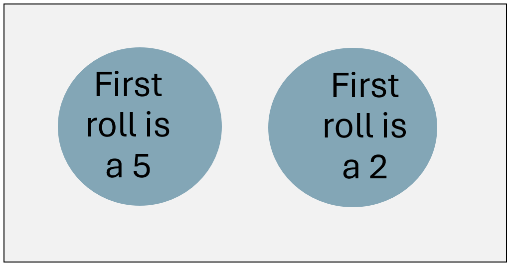
This time, the circles have no intersection (don’t overlap) because a first roll can’t be both a 5 and a 2. When two events have no intersection, they are said to be disjoint.
So, to calculate the probability of getting a 5 or a 2 on the first roll, we add the probability of getting a 5 to the probability of getting a 2. Since P(roll a 5) = 4/36, and since P(roll a 2) = 1/36, then the probability of rolling a 5 or a 2 on the first roll is calculated like this:
P(rolling a 5 or rolling a 2)
= P(roll a 5) + P(roll a 2)
= 4/36 + 1/36
= 5/36
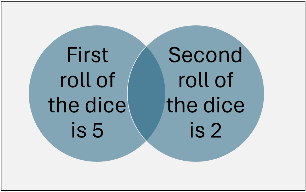
2) “What’s the probability of rolling a 5 on the first roll or a 2 on the second roll?” We can use the Venn diagram:
Notice that this time, the events have an intersection (the shaded area). This area represents the probability of that intersection. It represents all two rolls of the dice such that the first roll is a 5, and the second roll is a 2. Also, notice how the intersection is common to both events. So, when we calculate the probability of this question, we add the probabilities for both events and then subtract the intersection because, if we don’t, we would include the probability for the intersection twice.
So, P( 5 on the first roll or 2 on the second roll)
= P(5 on the first roll) + P(2 on the second roll) – P(5 on the first roll and 2 on the second roll)
Since we don’t yet have a way to calculate P(5 on the first roll and 2 on the second roll), we will simply state the rule, and then discover how we calculate it in the third question.
If we let A be an event, and B be an event, then we have the following rules for P(A or B)
If events A and B have no intersection, then
P(A or B) = P(A) + P(B)
If events A and B have an intersection, then
P(A or B) = P(A) + P(B) – P(A and B)
3) “What’s the probability of rolling a 5 on the first roll and a 2 on the second roll?”, we see that the the intersection (overlap) of the circles in the Venn diagram represents this event because it contains the outcomes of rolling the dice twice and having 5 on the first roll and a 2 on the second roll:
So, how do we find this probability? To answer this, we first need to consider whether the outcome of one of the events contributes to the outcome of the other event. In other words, we need to know if one event is dependent or independent of the other event.
Note: Just because the two events have an intersection does not by itself say whether the two events are dependent or independent. However, disjoint events (events that have no intersection) are dependent events. We will see why this is true in a bit. First, we need to look at conditional probability and independence of two events.
Conditional Probability and Independence of two events
Consider the Venn diagram:
The intersection of the two events represents all outcomes of two rolls of the dice such that the first roll produces a 5, and the second roll produces a 2.
To get that probability, lets ask the question “What’s the probability that the second roll produces a 2, given that the first roll is a 5?” These types of questions are known as conditional probabilities. How would we go about determining this probability?
We are asking for a probability of some event B given that the event A has already occurred. We use the following notation for such questions:
P(B|A)
We read this as “The probability of B given that A has occurred”. In the Venn diagram below, we can let A represent the event that the first roll is a 5, and B can represent the event that the second roll is a 2.
So, looking at the above Venn diagram, if the event A has occurred, we can think of the probability of B being the part of B contained in A. In other words, the intersection (the overlap which we refer to as A and B) represents the probability of B when we restrict our universe to the event A. However, if we restrict our universe to A, then we measure the intersection with respect to the measure of A. This gives us the formula for conditional probability:
Conditional Probability

So, now we can apply this formula to get the probability of rolling a 2 on the second roll, given that we rolled a 5 on the first roll:

Independence of two events
Now, let’s use the formula for conditional probability to answer question 3, “What’s the probability of rolling a 5 on the first roll and a 2 on the second roll?”
First, we will re-write the formula for conditional probability by multiplying both sides by P(A) to get

Let’s put P(A and B) on the left side of the equal sign so that we can keep track of things:

Notice that if the event A has no effect on the event B, then P(B|A) is simply P(B).
So, for two events A and B, A is independent of B (or B is independent of A) when

We can re-write this so that it’s easier to remember:
Probability of A and B occurring when A and B are dependent:
Probability of A and B occurring when A and B are independent:

The second formula also says that, when the probability of the intersection of two events is equal to the product of the probabilities of each of those events, then the events must be independent of each other.
If two events are not independent, then they are dependent. When events are dependent, the occurrence of one event affects the occurrence of the other event.
Consider two disjoint events C and D (no intersection). If we consider the formula for conditional probability

we see that the probability of the intersection on the right side of that formula must be equal to zero because there’s no intersection. So, the fraction on the right side will be equal to zero (providing that P(C) is not equal to zero). This gives us
P(D|C) = 0
This says that the probability of the event D given that C occurs is zero. So, if C occurs, then D doesn’t. This implies that the occurrence of D is affected by the occurrence of C. This means that the events C and D are dependent events. From this we see that, if two events C and D have no intersection, then they must be dependent events.
Now applying the conditional probability formula to question 3, “What’s the probability of rolling a 5 on the first roll and a 2 on the second roll?”, we get
P(5 on the first roll and 2 on the second roll) = P(2 on the second roll | 5 on the first roll) * P(5 on the first roll)
We think to ourselves, does the first roll of the dice have any effect on the second roll of the dice? No, it doesn’t. So, P(2 on the second roll | 5 on the first roll) becomes P(2 on the second roll), and now we get
P(5 on the first roll and 2 on the second roll) = P(2 on the second roll) * P(5 on the first roll)
We can also write it this way:
P(5 on the first roll and 2 on the second roll) = P(5 on the first roll) * P(2 on the second roll)
Now, all we need to do is determine P(5 on the first roll) and P(2 on the second roll).
Since there are 4 equally likely rolls of the dice which total to 5, and only one possible outcome for rolling a 2, and since there are 36 equally likely outcomes for one roll of a pair of dice, we have
P(5 on the first roll) = 4/36
P(2 on the second roll) = 1/36
Hence,
P(5 on the first roll and 2 on the second roll) = 4/36 * 1/36 = 4/1296 = 0.0030864198 (approximately).
Calculating The Probability for “At Least One”
This calculation happens when we want to obtain the probability that, among several trials, we get at least one occurrence of some event. Consider a pair of dice. What’s the probability that, out of 4 rolls of the dice, at least one of those rolls is a 7? The trick to getting this probability is to think about what this question implies. Out of the four rolls we could have one 7, two 7’s, three 7’s, or all four be 7’s. The only possibility left for four rolls of the dice when it comes to rolling a 7 is no 7’s among the four rolls of the dice. So, we compute the probability by realizing that, given all possible outcomes of 7 for the four rolls of the dice is the universe that we’re concerned with, then 1-P(no 7’s in four rolls) gives us the probability of at least one 7 in four rolls of the dice. Since the probability of rolling a 7 is 6/36, the probability of not rolling a 7 is 1 – 6/36 = 30/36 = 15/18. Then, the probability of not rolling a 7 on four rolls of the dice is (15/18)*(15/18)*(15/18)*(15/18) = 0.4822530864. So, the probability of getting at least one 7 in four rolls is 1 – 0.4822530864 = 0.5177469136.
5.4 – Contingency Tables and Probability Trees
Contingency Tables
With the rules for computing probability, we can now organize data for two categories into two-way tables called contingency tables.
A random sample of 120 Renton Technical College students and 120 University of Washington students gives us the following contingency table. The categories are “Employment Post-Graduation” (this category has two sub-categories, “Employed Full-Time Post Graduation” and “Not Employed Full-Time Post Graduation”) and “School” (this category has two sub-categories, “RTC Students” and “UW students”)
| Employment Post-Graduation/School | Employed Full-Time Post Graduation | Not Employed Full-Time Post Graduation | |
| RTC Students | 92 | 28 | 120 |
| UW Students | 76 | 44 | 120 |
| 168 | 72 | 240 |
This allows us to ask questions such as:
1) What percentage of RTC students will be employed full-time post graduation?
To answer this question, we must realize that we’re restricting our attention to the row for RTC students. This is the same thing as a conditional probability. We’re looking to find
P(Employed full-time post graduation | RTC Student)
There are 120 RTC students in this sample. 92 of them are employed full-time post graduation. So, we create the fraction 92/120 because it represents the 92 employed students out of the 120 RTC students in this sample. Hence, 92/120 = 0.7666…, which when rounded to two decimal places is 0.77 or 77%.
2) What percentage of UW students will be employed full-time post graduation?
This is similar to the first question. Out of the 120 UW students, 76 are employed full-time post graduation. Hence, 76/120 = 0.6333…, which when rounded to two decimal places is 0.63 or 63%.
3) What percentage of all the students in this sample are RTC students and employed full-time post graduation?
Notice the wording in this question. We want the percentage of all students (both schools) who are both RTC students and employed full-time post graduation. This gives us the fraction 92/240 = 0.38333…, which when rounded to two decimal places is 0.38 or 38%.
4) What percentage of students not employed full-time post-graduation are UW students?
Notice now that we’re restricting our attention to those students who are not employed full-time post graduation. There are 72 students who are not employed full-time post graduation. Out of that number there are 44 UW students. So, 44/72 = 0.61111…, which when rounded to two decimal places gives us 0.61 or 61%.
5) What percentage of all students in the sample are not employed full-time post graduation?
For this question, we want the percentage of all students (both schools) who are not employed full-time post graduation. Hence, 72/240 = 0.3 or 30%.
Contingency tables are often created using a random sample. In the table above, the sample size is 240. As we will see soon, a random sample will allow us to estimate the probability for the greater population. The important thing to notice at this time is when the rows percentages (or the column percentages) are “close”, then the two categorical variables are independent of each other. The row percentages are the percentages that we get from the fractions of the totals for the rows. The column percentages are the percentages that we get from the fractions of the totals for the columns.
Row Percentages
| Employment Post-Graduation/School | Employed Full-Time Post Graduation | Not Employed Full-Time Post Graduation | |
| RTC Students | 92/120 = 77% | 28/120 = 23% | |
| UW Students | 76/120 = 63% | 44/120 = 37% | |
Column Percentages
| Employment Post-Graduation/School | Employed Full-Time Post Graduation | Not Employed Full-Time Post Graduation | |
| RTC Students | 92/168 = 55% | 28/72 = 39% | |
| UW Students | 76/168 = 45% | 44/72 = 61% | |
It doesn’t matter whether we use the row percentages or the column percentages to see if the two categorical variables are independent of each other. Looking at the row percentages, it’s easy to see that the percentages in the RTC Students row are different than the corresponding percentages in the UW Students row. How different? It turns out that the degree to which the different percentages indicate independence will be related to the sample size. We’ll see this later in the course.
It’s important to realize that the percentages in a contingency table can be understood to be approximations to the true percentages in the populations of RTC and UW. Why an approximation? Because the 240 students (120 RTC students and 120 UW students) are a sample.
We can now think about the percentages in the contingency table as approximations to the respective probability of randomly selecting any of the categories, subcategories, or intersections. For example, the percentage of RTC students employed full-time post-graduation is 92/120 = 0.77 (rounded to two decimal places). This percentage is an approximation to the probability of randomly selecting a graduated RTC student who is working full-time.
Probability Tree
A probability tree is another way to express probabilities by following a path along the tree. Here’s the same information as the contingency table we first looked at expressed as a probability tree:
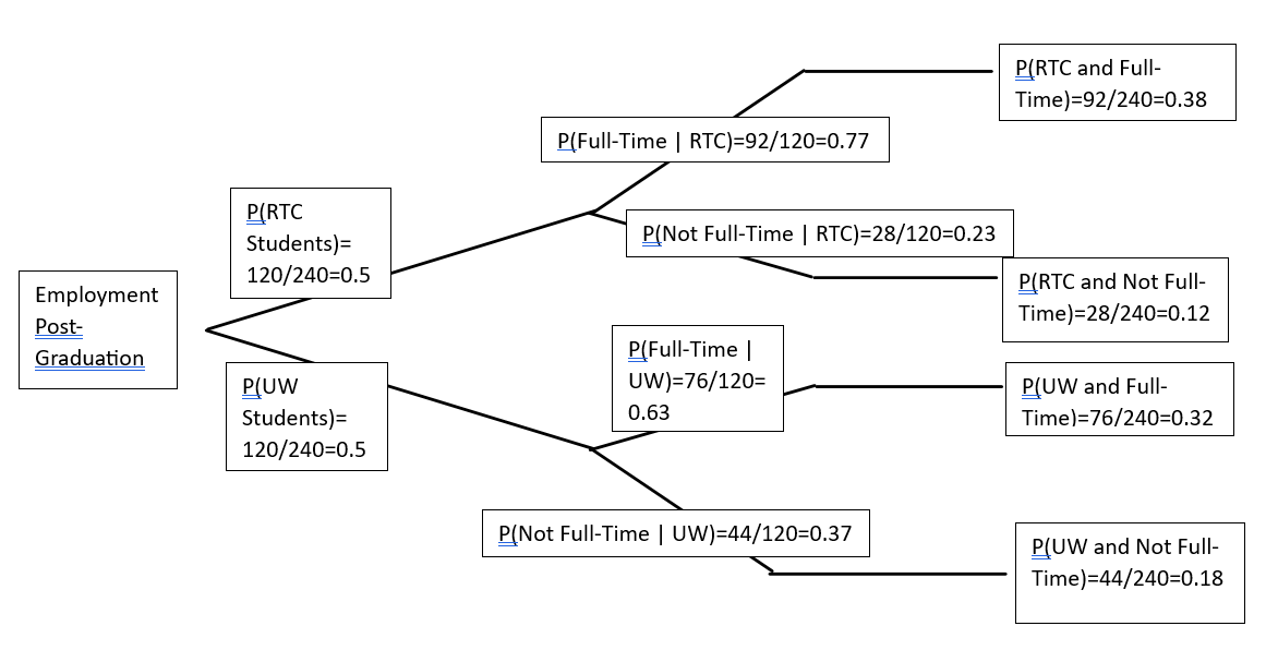
The first branching on the left shows the probabilities for RTC and UW (out of the 240 total number of students in this sample). The second branching shows the conditional probabilities, i.e., the probability given the path they came from on the first branching. At the end of the branches on the right are the probabilities of each possible intersection of the categories. These probabilities are called the leaves of the tree because they’re at the end of the branches.
Notice that the probabilities for the intersections are the product of the probabilities of the first and second branches. For example the probability of UW and Full-Time is 76/240. This is the product of the probability of selecting a UW student in the sample (120/240) and the probability of working full-time given we selected a UW student (76/120). To see this we multiply (120/240) * (76/120) = 76/240.
Another thing to notice is that the sum of all the leaves is 1. This is because the intersections of the categories are disjoint and make up all the possible events in the contingency table.
Probability is the chance that something happens. Probability is always a number 0 through 1, possibly being equal to 0 or 1. We can also express a probability as a percentage 0% through 100%, possibly being equal to 0% or 1%.
Outcomes are events that can't be broken into separate events. Considered by themselves, they are events, and any collection of them make up events. Each outcome is distinct from any other outcome. The use of the word "outcome" is sometimes used to mean the result of some event. We must take care to distinguish between the colloquial use of the word and the use of the word with respect to a probability space.
The collection of all possible outcomes for some population of things or people. It has the same meaning as "probability space".
The collection of all possible outcomes for some population of things or people.
