6.1 – The Normal Model

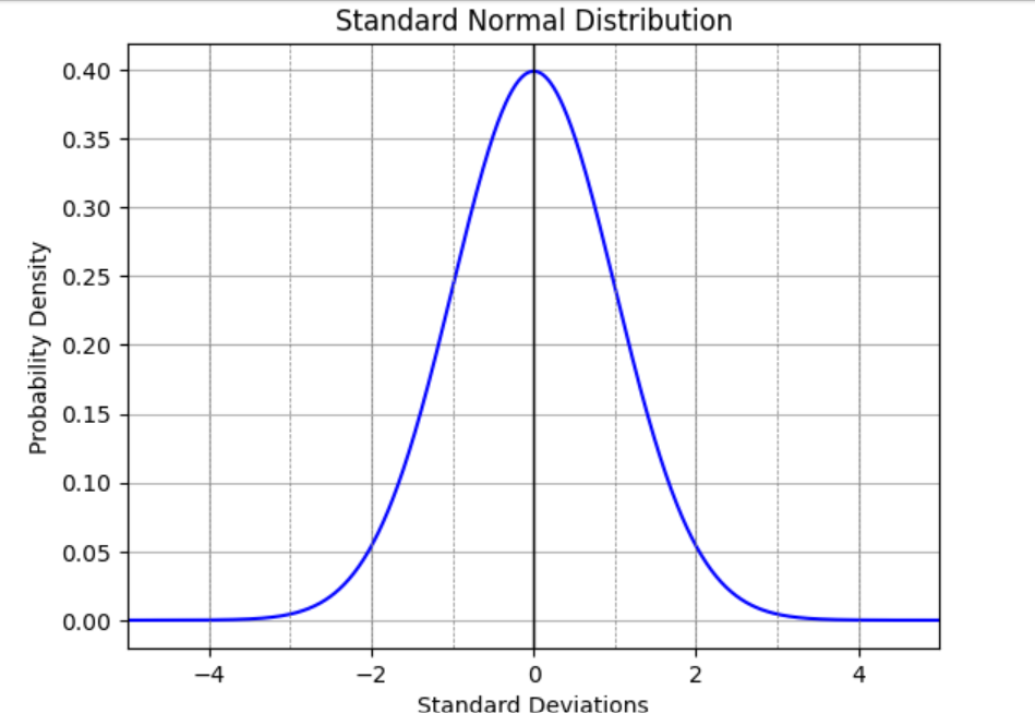
The Normal model is central to statistics. Without it, modern statistics would not exist. The Normal model is a distribution of data values along a number line with a bell-shaped curve above that number line indicating where the data values are concentrated. Some of the histograms we saw in chapter 4 have an outline to which we can fit a Normal model.

Things to know about a Normal model:

• It’s a math model that we use to get information from histograms that have the same shape.
• It’s a function which is plotted on a grid using a horizontal and vertical axis.
• The left and right parts of the graph are called the tails. The left and right tails extend to negative and positive infinity respectively. They get closer and closer to the horizontal axis but never touch it.
• Between any two points on the horizontal axis, the area  under the curve and between those two points represents some probability. The area under the entire curve from negative infinity to positive infinity is equal to 1.
• The Standard Normal model has the horizontal axis marked off in units of standard deviations. Its mean is zero, and its standard deviation is 1.

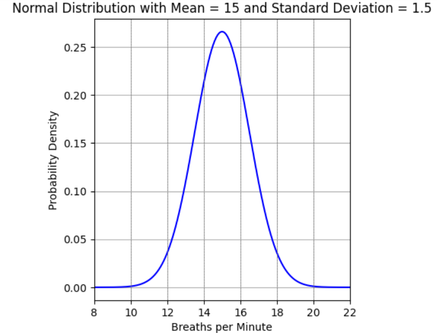
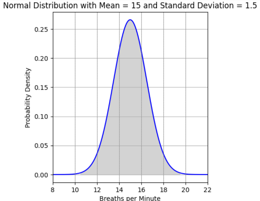
• Normal models can have the horizontal axis marked in whichever units are being used. In the Normal model below, we use units of breaths per minute.

Empirical Rule For The Normal Model; The 68-95-99.7 Rule

Every Normal model has the following properties:

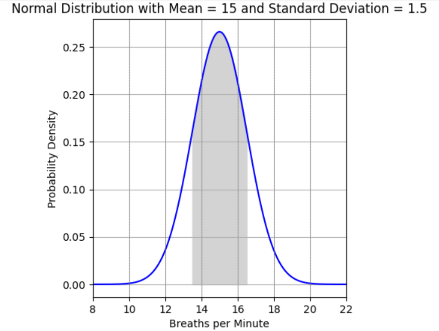
• The area under the curve and between 1 standard deviation below the mean and 1 standard deviation above the mean is approximately the middle 68% of the total area. Note that the area in the Normal model below is shaded between 13.5 and 16.5. Since the standard deviation is 1.5, 1 standard deviation below 15 is 13.5. Similarly, 1 standard deviation above 15 is 16.5.

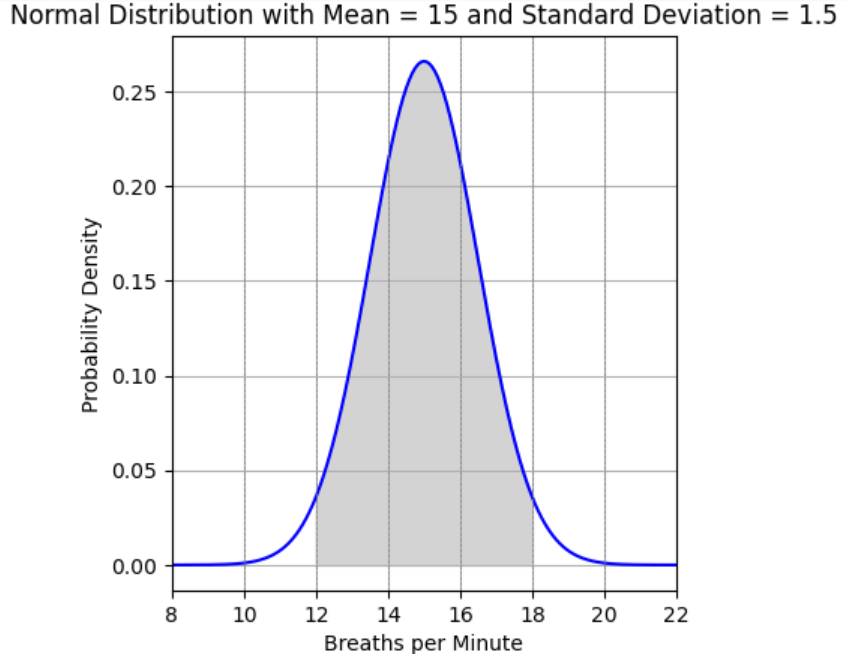
• The area under the curve and between 2 standard deviations below the mean and 2 standard deviations above the mean is approximately the middle 95% of the total area. Note that the area in the Normal model below is shaded between 12 and 18. Since the standard deviation is 1.5, 2 standard deviations below 15 is 12. Similarly, 2 standard deviation above 15 is 18.

• The area under the curve and between 3 standard deviations below the mean and 3 standard deviations above the mean is approximately the middle 99.7% of the total area. Note that the area in the Normal model below is shaded between 10.5 and 19.5. Since the standard deviation is 1.5, 3 standard deviations below 15 is 10.5. Similarly, 3 standard deviation above 15 is 19.5.

Area Under The Normal Curve Between Any Points

If we want to find the area under the Normal model between any two points or from a point all the way to negative infinity or positive infinity, we need to use a Normal calculator. The TI-84 or Excel can do this. Here are some examples with the keystrokes for both technologies:

Example: Given a Normal model with mean of 15 breaths per minute and standard deviation of 1.5 breaths per minute, find the probability that we randomly select a person whose resting breaths per minute is less than 12.

Solution:

Here are the keystrokes for the TI-84:

2nd, VARS, 2: normalcdf, lower: -1E99 (use the “(-)” key for the negative sign), upper: 12, Mu (mean): 15, sigma (standard deviation): 1.5, scroll down to Paste and click ENTER twice. We see that the probability is 0.023 (rounded to three decimal places).

Here are the keystrokes for Excel (first click in an empty cell):

Formulas, More Functions, Statistical, NORM.DIST, X: 12, Mean: 15, Standard_dev: 1.5, Cumulative: TRUE. We see that the probability is 0.023 (rounded to three decimal places).

Example: Using the 68-95-99.7 rule, find the probability of randomly getting a person whose resting breaths per minute is between 15 and 16.5.

Solution:

We remember that, for a Normal model, we have 68% of the probability between 1 standard deviation below the mean and 1 standard deviation above the mean. Since a Normal model is symmetrical about its mean, and since we need to find the probability between the mean of 15 and 16.5, which is one standard deviation above it, we divide 68% by 2 to get 34%.

Example: Using the 68-95-99.7 rule, find the probability of randomly getting a person whose resting breaths per minute is between 12 and 13.5 breaths per minute.

Solution: We remember that, for a Normal model, we have 95% of the probability between 2 standard deviation below the mean and 2 standard deviation above the mean. Since a Normal model is symmetrical about its mean, and since we need to find the probability between 12 (which is 2 standard deviations below the mean) and 13.5, which is one standard deviation below the mean, we first subtract 68% from 95%, and then divide this result by 2 to get 13.5%.

NOTICE: We got an answer of 13.5%. This is a probability. However, it looks like the 13.5 breaths per minute. Don’t confuse the two! The answer just happens to look like another value in the problem.

Normal Percentiles

A Normal percentile is simply the value which has a particular percentage of the area under the Normal curve to the left of it.

Example: For a Normal model with mean 7.1 meters and standard deviation of 1.4 meters, the 67th percentile is the value that has 67% of the area under the curve to the left of it. We can find this value by using the TI-84 or Excel.

Here are the keystrokes for the TI-84:

2nd, VARS, 3: invNorm, area: 0.67, Mu (mean): 7.1, sigma (standard deviation): 1.4, then scroll down to Paste and click ENTER (you might have to click ENTER twice). We see that the 67th percentile for this Normal model is 7.7159 (rounded to four decimal places).

Here are the keystrokes for Excel (first click in an empty cell):

Formulas, More Functions, Statistical, NORM.INV, Probability: 0.67, Mean: 7.1, Standard_dev: 1.4, OK. We see that the 67th percentile for this Normal model is 7.7159 (rounded to four decimal places).

ChatGPT

Using your ChatGPT account, ask it 3 questions about what we’ve learned so far.

6.2 – What Questions Can We Answer About A Population Mean Given Some Data?

The mean of any population at some point in time can be estimated using the techniques we will develop in this chapter. We have to keep in mind a few things:

• A mean or average is for quantitative data, i.e., data that uses units. Be sure to understand that the techniques in this chapter are for quantitative data, not counts of a category. Counts and proportions will be dealt with in the next chapter.
• We estimate the mean of a population by first taking a random (or suitably representative) sample which gives us a sample mean. This sample mean is called a point estimate. It’s the simplest way to estimate the mean of the population.
• Sample means vary from sample to sample. We can think about the histogram of all the possible sample means for a population. This histogram will have a bell shape outline as long as the sample size is big enough. It turns out that, if the population from which we draw our sample has a bell shape distribution, then even for small sample sizes, the shape of the histogram of all sample means of some size n drawn from that population will also have a bell shape distribution. In general, the further the shape of the histogram of the individual values in a population, the larger the sample size needs to be to make the shape of the histogram of the sample means bell-shaped.

Below the instructions (1 through 11) is an interactive which demonstrates how a sampling distribution of the mean works. Here’s what to do to see what happens when we make a histogram of sample means of different sample sizes:

1. Notice on the left side of the interactive below that the population from which we will draw our samples is bell-shaped. In fact, it’s a Normal model. The Normal model plays a central role in statistics. We will discuss this more in a bit.
2. In the upper right part of the interactive you should see a check-box next to “Show Sampling Options”. Click that box. It should make other things appear.
3. Below “Show Sampling Options” you should see “Number of samples”. Make the number in that box 10000. This is how many samples we we take of some specified size.
4. Below that is “Sample size”. Make that 2. This is the size of each of the 10000 samples. In other words, this app will randomly sample 2 values from the distribution of the population indicated on the left side of the screen.
5. On the lower right side, make sure that “Rescale” is checked.
6. There are two sets of axes. Watch what happens on the right-most axes as you repeatedly click the “Draw Samples” button below “Number of samples”. Click “Draw Samples”.
7. Now, at the bottom right, click the box next to “Overlay Normal Distribution”.
8. Notice how closely the overlay of the Normal model (the curve) fits the outline of the histogram.
9. Next, uncheck “Overlay Normal Distribution” and go back to the left side and click the drop-down menu for “Population shape”. Select “Skewed right”.
10. Now, click “Reset” (next to “Sample size”) and click “Draw Samples”. Notice that, this time, the histogram of those sample means retain some of the shape of the skewed-right distribution. Click “Overlay Normal Distribution”. Notice that it doesn’t fit that well.
11. Now, uncheck “Overlay Normal Distribution”, change “Sample size” to 30, and click “Draw Samples”. Notice that the histogram looks more symmetric and bell-shaped than it did when we used a sample size of 2. This is a very important thing to notice. As it turns out, as the sample size gets larger, the sampling distribution becomes more Normal shaped.

• The special properties of the Normal distribution discussed above allow us to determine probabilities of events that follow this type of distribution.
• Given one randomly obtained sample, its mean and its standard deviation, we can infer how much spread about that sample mean we need so that we can be confident that such an interval contains the population mean. This is the essence of the classic statistical tool called a confidence interval. We will develop this technique in a bit. First we need to prepare some essentials.