Chapter 8: Microsoft® Excel®

What We’ll Cover >>>

• Spreadsheet/Financial Software
• Microsoft Excel
• Worksheet Formatting and Inserts
• Workbook Design
• Datasets
• Tables
• Calculations
• Charts and Graphs
• Review and Distribution

Spreadsheet software allows users to create, edit, and print financial information and data organization. The software enables you to add data, store it electronically, display it on a screen, modify it by entering commands and characters from the keyboard, and print it.

Financial software and spreadsheets has evolved into much more than just sheets of data. One can have thousands of records to be analyzed, calculated, summarized, and expressed for reporting in graphs, charts, and data dashboards. It also allows to import of big data, and export of content for other databases, like sales contacts, marketing management applications, etc. Modern spreadsheet software is integrated into the cloud so that data can be accessed from cloud-based storage.

Spreadsheet/Financial Software

A spreadsheet is a file with cells in rows and columns that allow you to arrange, calculate and sort data. Data in a spreadsheet consists of numeric values, text, formulas, references and functions. Spreadsheets are used to visualize data in a meaningful way that can be used to make complex decisions. Spreadsheets can take raw data, and tell a story with it.

Spreadsheet software can be part of an integrated suite of tools, or be stand-alone. It can be installed on a computer for full and robust features and integration with other resources; it can be accessed on the web in a light format, and it can be a basic utility tool, like text editing applications. Some programs/suites are payware, such as those used in many workplaces; others are shareware or freeware. Information in this chapter should offer you transferrable skills for use in any word processing application.

Common Spreadsheet Software

• Apple Numbers Online: Part of the iWork productivity suite and operates on the MacOS, iPadOS, and iOS operating systems. Users feel that it is an easy-to-use application that allows them to quickly create spreadsheets on their Apple devices.
• Google Sheets: Online: Included as part of a free, web-based software office suite offered by Google within its Google Drive service. Allows users to create, view, and edit files online while collaborating with other users in real-time. Available as a web application supported on Google Chrome, Mozilla Firefox, Internet Explorer, Microsoft Edge, and Apple Safari web browsers. Compatible with Google Drive.
• Microsoft Excel: Commercial: Operates on Windows and Mac. Part of Office 365 Recent features include robust formulas and functions, charts, graphs, and sparklines.
• Smartphone apps that allow for quick use and editing on-the-go.
• Spreadsheet apps in free/open source office suites.

Microsoft Excel

Since Microsoft Excel is widely used in business settings, and since we are using Microsoft Windows, we will focus on Excel going forward. There are many similarities in tools and functions across spreadsheet software, so the skills we are learning can be translated to other software and apps. The following Try Me activities are designed to be completed using Microsoft Excel in Office 365 on a PC with Windows 10 or higher.

We will use Excel to perform complex calculations, analyze data so that we can make intelligent decisions, and create visually interesting charts and graphs that help us understand the data. Since Excel is used for Data Analysis, it is best to use a keyboard and mouse or touchpad rather than the touchscreen.

Accessing Excel

• In your Computer, use the relevant start menu to open MS Excel (look for little green icon). On a PC this is a start button on the keyboard, and/or menu on the lower left of the screen. On a Mac, this should be in the top-screen Menu option.
• Excel will open with options to create a blank workbook, open an existing file, and use templates.

DEMO EXAMPLE follow-through

• Locate Excel on your computer. This can be done with your computer’s search tool so that you can locate the application icon.
• Click Microsoft Excel icon/execution file to launch the Excel application where you are presented with workbook options to help get you started.
• Options will include a Blank workbook, tours of program information, templates installed with your application, and the choice of opening an existing Excel file.
• New Excel workbooks start with a blank file of worksheet(s) tabbed pages for you to start new work.
• Existing files can be opened from your computer, an external drive, and an online source like OneDrive (if you have/use that).
• Choose Blank Workbook, which will open a new, blank workbook with a default of 3 Sheet tabs.

The User Interface (UI) menus

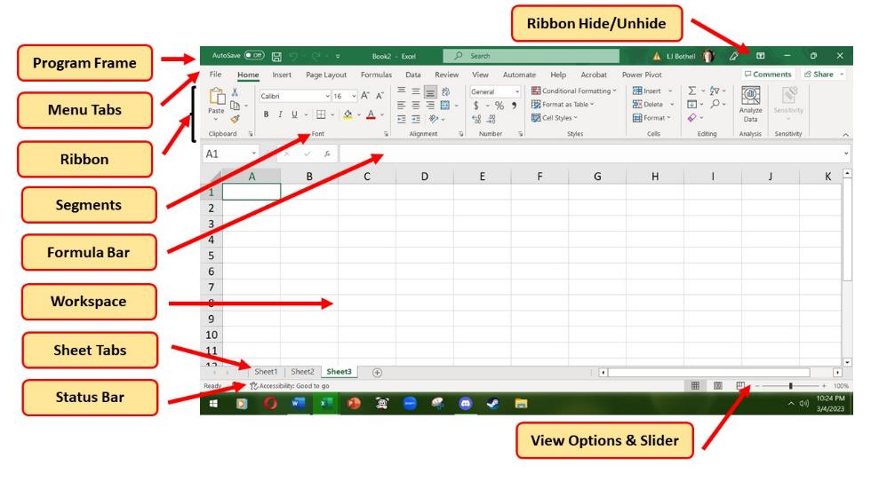
MedAttrib: author-generated. MS Excel user interface.

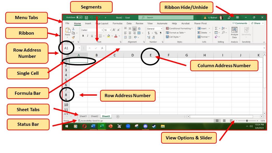
• Place your mouse pointer over cell A1 and click.
• Check to make sure column letter A and row number 1 are highlighted.
• Look at the application’s upper left field (below the ribbon) where you should see A1 in the Name Field.
• Move the mouse pointer to cell D6.
• Click and hold the left mouse button and drag the mouse pointer back to cell A1.
• Release the left mouse button. You should see several cells highlighted.

This is referred to as a cell range and is documented as follows: A1:D6. Any two cell locations separated by a colon are known as a cell range. The first cell is the top left corner of the range, and the second cell is the lower right corner of the range. This is important because cell ranges will be an important part of formulas later on.

Keyboard Shortcuts > Worksheet Navigation.

• Use the arrow keys on your keyboard to activate cells on the worksheet.
• Hold the SHIFT key and press the arrow keys on your keyboard to highlight a range of cells in a worksheet.
• Hold the CTRL key while pressing the PAGE DOWN or PAGE UP keys to open other worksheets in a workbook.
• MAC Users: Hold down the FN and CMD keys and press the left or right arrow keys

In Excel, the user interface contains several menu tabs (tab, menu), with ‘Ribbons’ (ribbon) that display icons (like buttons) with text descriptions of various activities related to a task. On a ribbon, you will often see groups (group) of icons for tasks that relate to one another, like the Home ribbon’s Font group, Paragraph group, etc. Some of these icon buttons will do a simple task in one step, while others may open a panel (panel) which is a detailed, multi step or tab window of options. Sometimes you may instead see a context dropdown (dropdown) menus of options, or a dialog box (dialog) with a couple of fields to complete.. Shown (in the program’s order) are:

Explore Menu/Ribbon tabs:

• File: Accesses the program backstage area for various options. Set your preferences for workflow and productivity.
• Home: Basic text functions –  formatting, positioning, styles
• Insert: tables, images, shapes, charts, page sections
• Page Layout: Layout of the slides – margins, positioning, indents, etc.
• Formulas: For performing mathematical calculations on rows and columns of numerical data.
• Data: For sorting and organizing data.
• Review: Spelling, language, tracking, etc.
• View: screen views, rulers, gridlines, windows.
• Add–ins: Based on additional programs a workplace might have that work with MS Excel. Can include types of macros and specific formulas.
• Additional add-in/specialty tab menus: These are dependent on having MS Word-related add-ins like Acrobat, Power Pivot, etc.
• Contextual tab menus: These are contingent on a specific item in the program’s workspace being activated. For instance, clinking on an image, table, or header / footer will activate a context menu/ribbon on the right side of the UI that shows a menu dedicated to actions that can be done specifically for the active item (picture editing).

We’ll cover more detail on specific Menu toolbar ribbons in the following demo sections.

In addition to the ribbon and Quick Access Toolbar, you can also access many commands by right clicking anywhere on the worksheet, which will enable a dropdown menu of choices that are relevant to what you need to accomplish.

MAC Users: There is no “Right-click” option for Excel for Mac. Instead, hold down the control key and click the mouse button.

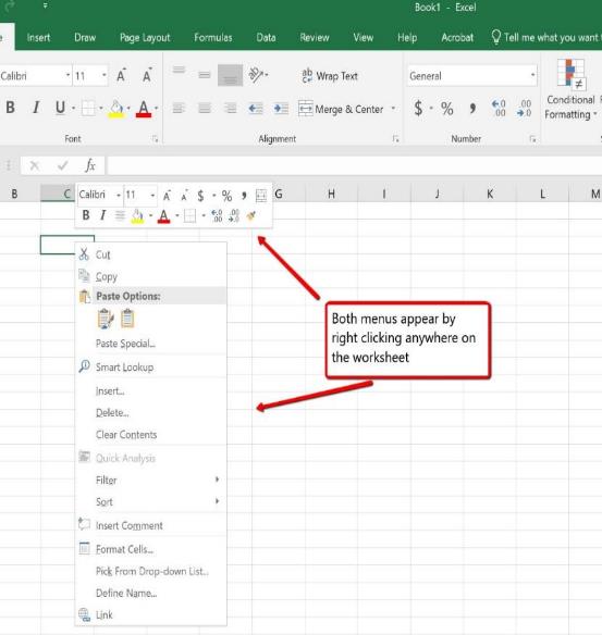
MedAttrib: Beginning to Intermediate Excel. MS Excel’s Right-Click dropdown menu.

Worksheets

Worksheets are the Excel equivalent of the Word document. A worksheet is made up of are made up of a tabular view of cells, rows, and columns. Their common MS Excel file extension is .xlsx. They can contain:

• Text data.
• Calculations.
• Inserted items like images, graphs, and tables,
• Page breaks, print area settings

Views – View Tab

• You can see different views as part of the main interface – lower right-hand side of the user interface, and also from the View tab’s ribbon.
• You can set rulers on or off.
• You can also set guides for aligning text and images.
• You can choose the window view you like to work in, such as normal, page break, page layout, and print layouts.

Preferences – File tab

You can set your Excel program preferences for documents and program workflow, for smoother productivity, in the ‘backstage’ area of the program.

• Same layout as PowerPoint, Word, and Access.
• Allows personalizing, print, save, and publish settings.
• Preferences: Excel Options:
• Customize editing, saving, and other program options.
• Personalize a mini-toolbar so you can minimize the ribbon.

The Work stage

• Excel opens with a default number of blank workbook pages, which you can change, name, and delete. You can also change the default number in the program options.
• Cells are all named by column (letter) and row (number).
• Data entry goes into individual cells, and is accepted (enter) or rejected (red check).
• The Formula bar at top shows data that is inside a specific cell, as well as details of any calculation formula when used.
• Calculations are based on selecting various cells and their to be calculated in some way.
• Cells can be formatted like in Word: font family, font color, font size, cell contents alignment, etc.
• The worksheet ‘page’ can be formatted with borders, color, and alignment of objects.

In Excel, all input data for sorting, filtering, calculation, and analysis is stored in a cell. Cell content is anything that is stored in the cell and can be either a constant value or a formula. The most commonly used values are text values (string of text like a customer’s name or phone number) and number values (like a count, etc.) We’ll cover more on this in the Datasets section of this chapter.

• A text value is also referred to as a label. It is not something to calculate, which is why a phone number or social security number is considered ‘text’.
• A numeric value can actual numeric data, like a date, item of currency, a percentage, etc. These can have specific numeric formats added to them, like short date, a percentage format, a dollar sign, decimal points, etc. This is not the same as changing a number to ‘look’ like a phone number. Numeric values can be calculated.
• Calculations in a cell are when content from one or more calculatable cells are used in a formula to get an answer. An example would be the sum of the numeric values in a couple of cells to give a total amount.

MedAttrib: author-generated. MS Excel cells, rows, and columns.

ACTION: MS Excel Try Me Activity #1

• Follow along and try things. There is no “wrong”, this is just play and exploration! This is what we will create:

MedAttrib: author-generated. MS Excel cells, rows, and columns.

Plain Data

• BEFORE you do this activity, make sure you have taken the Preparation Steps in the Part 1 Introduction (creating file directories and folders for all your work in this book). This allows you to have a safe place to save your files of work while you explore this content.
• Create a new, blank workbook in Excel.
• Immediately give it a name and save it to your Examples on your computer. File naming recommendation: Excel_dataentry.xlsx.
• Click cell A2.
• Type your first name and press the ENTER key. After you press the ENTER key, cell A3 will be activated. Using the ENTER key is an efficient way to enter data vertically down a column.
• Enter the following first names, pressing ENTER after each: Alfre, Jonna, Patrick, Julio, Ajay
• Click cell B2.
• Type your last name and press the ENTER key. After you press the ENTER key, cell B3 will be activated.
• Type names into cells B3 and press the ENTER key. Do this through Cell B7. Names: DuShayne, Mills, McNeill, Mendez, Bashira
• Click cell C2.
• Type the number 50 and press the ENTER key.
• Enter the following numbers in cells C3 through C7: 75, 22, 180, 65, 48, 125
• SAVE your work: CTRL S. MAC Users: CMD S.

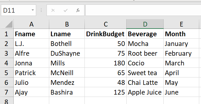
Column Headings

In Excel, data rarely means anything to a viewer if there is no context attached to it. Commonly this is done through column headings, which identify what the content in the column is supposed to be. This can also be done as row headers instead, but in this course we’ll mostly use the standard column headings.

In the image above, you can see a row of bold text in cells A1-C1. These are column headers, and you can type them:

• In cell A1, type Fname, then press TAB. Tab lets you move to the right of an active cell and activate the next one for data entry.
• In cell B1, type Lname and press TAB.
• In cell C1, type Coffee budget, and press TAB.

These are the column headings that tell you the first column is full of first names, the second column is full of last names, and the third column has amounts for a coffee budget.

Editing Data

Data that has been entered in a cell can be changed by double clicking the cell location or using the Formula Bar. You may have noticed that as you were typing data into a cell location, the data you typed appeared in the Formula Bar. The Formula Bar can be used for entering data into cells as well as for editing data that already exists in a cell. The following steps provide an example of entering and then editing data that has been entered into a cell location:

• Click cell D2 in the Sheet1 worksheet.
• Type Moc and press the ENTER key.
• Click cell D2.
• Move the mouse pointer up to the Formula Bar. You will see the pointer turn into a cursor. Move the cursor to the end of the abbreviation Moc and left click.
• Type the letters ha to complete the word Mocha.
• Click the check mark to the left of the Formula Bar. This will enter the change into the cell.
• Use this method – clicking a cell but typing into it through the Formula Bar – to add coffee beverages into cells D3-D7.
• Use this method to also add the data FaveDrink into cell D1 (the header for this column).
• SAVE your work: CTRL S / MAC CMD S.

Keyboard Shortcut: Editing Data in a Cell. Activate the cell that is to be edited and press the F2 key on your keyboard.

Autofill

The Auto Fill feature is a valuable tool when manually entering data into a worksheet. This feature has many uses, but it is most beneficial when you are entering data in a defined sequence, such as the numbers 2, 4, 6, 8, and so on, or nonnumeric data such as the days of the week or months of the year. The following steps demonstrate how Auto Fill can be used to enter the months of the year in Column E:

• Click cell E2 in the Sheet1 worksheet.
• Type the word January and press the ENTER key.
• Click cell E3 and type February, then Press Enter.
• Click cell E4 and type March, then Press Enter.
• Move the mouse pointer to the lower right corner of cell E4. You will see a small square in this corner of the cell; this is called the Fill Handle. When the mouse pointer gets close to the Fill Handle, the white block plus sign will turn into a black plus (+) sign.
• Left click and drag the Fill Handle through cell E13. Notice that the Auto Fill tip box indicates what month will be placed into each cell. Release the mouse button when the tip box reads “December.”

Once you release the left mouse button, 12 months of the year should appear in the cell range E2:E13. You will also see the Auto Fill Options button. By clicking this button, you have several options for inserting data into a group of cells.

• SAVE your work.

Deleting Data

There are several methods for removing data from a worksheet, and with each method, you use the Undo command if you change your mind. This is a helpful command in the event you mistakenly remove data from your worksheet.

You can delete data by selecting a cell and using your Delete keyboard button. You can right-click on a cell and choose Delete. You can select a cell and use the Home tab Editing group and choose the Clear icon, then Clear all.

• Select cells E8 through E13.
• Press the DELETE key on your keyboard. This removes the contents of the cells.
• MAC Users: Hold down the Fn key and press the Delete key
• Click the Undo button – which is by default available in the Quick Access Toolbar. This should replace the data in the cells E8-E13.
• Select cells E8 through E13.
• Use the Home tab Editing group and choose the Clear icon, then Clear all.
• SAVE your work: CTRL S / MAC CMD S.

Keyboard Shortcut: Undo Command: CTRL Z / CMD Z

Adjusting columns / rows

TIP: Column and Row Addresses. Every row has an address – the gray “cell” number to the left of the editable part of your worksheet. Evey Column has one too, the gray “cell” letter just above the editable part of your worksheet. You click on these to select a whole row or column.

There may be a few entries in a worksheet that appear cut off. This is because the column is too narrow for this word. The columns and rows on an Excel worksheet can be adjusted to accommodate the data that is being entered into a cell using three different methods. The following steps explain how to adjust the column widths and row heights in a worksheet:

• Bring the mouse pointer between the column number addresses of Column A and Column B in the Sheet1 worksheet (column address is the gray ‘cell’ just above Cells A1 and B1). You will see the white block plus sign turn into double arrows.
• Press your cursor down (press and hold your left mouse button when you click) so your can drag the column to the right until the entire column looks like it is about 2 inches wide. As you drag the column, you will see the column width tip box. This box displays the number of characters that will fit into the column using the Calibri 11-point font which is the default setting for font/size.
• Release the left mouse button.

You may find that using the click-and-drag method is inefficient if you need to set a specific character width for one or more columns. This is a second method for adjusting column widths when using a specific number of characters:

• Click any cell location in Column A. You can highlight cell locations in multiple columns if you are setting the same character width for more than one column.
• In the Home tab of the ribbon, left click the Format button in the Cells group.
• Click the Column Width option from the drop-down menu. This will open the Column Width dialog box.
• Type the number 29 and click the OK button on the Column Width dialog box. This will set Column A to this character width.

A third method is the double-click one:

• Once again bring the mouse pointer between Column A and Column B so that the double arrow pointer displays and then double-click to activate AutoFit. This features adjusts the column width based on the longest entry in the column.

Keyboard Shortcut: Column Width. Press ALT key on keyboard, then press letters H, O, and W one at a time. MAC Users: not available.

Row Height adjustment works similarly. Steps 1 through 4 demonstrate how to adjust row height, which is similar to adjusting column width:

• Click cell A1.
• In the Home tab of the ribbon, left click the Format button in the Cells group.
• Click the Row Height option from the drop-down menu. This will open the Row Height dialog box.
• Type the number 24 and click the OK button on the Row Height dialog box. This will set Row 1 to a height of 24 points. A point is equivalent to approximately 1/72 of an inch. This adjustment in row height was made to create space between the totals for this worksheet and the rest of the data.

Now, to adjust the row with the autofit option:

• Bring the mouse pointer between Row 1 and Row 2 at the row address (the 1 and 2 just to the left of Cells A1 and A2), so that the double arrow pointer displays, and then double-click to activate AutoFit. This features adjusts the row width based on the largest entry in the row.
• SAVE your work.

Keyboard Shortcut: Row Height. Press ALT key on your keyboard, then press letters H, O, and H one at a time. MAC Users: not available.

Hiding and unhiding columns / rows

In addition to adjusting the columns and rows on a worksheet, you can also hide them. This is a useful technique for enhancing the visual appearance of a worksheet that contains data that is not necessary to display but which is otherwise needed for computations and/or storage.

• Click cell C1.
• Click the Format button in the Home tab of the ribbon.
• Place the mouse pointer over the Hide & Unhide option in the drop-down menu. This will open a submenu of options.
• Click the Hide Columns option in the submenu of options. This will hide Column C.

Keyboard Shortcut: Hiding Columns. Hold down CTRL key while pressing number 0 on your keyboard.

To unhide a column, follow these steps:

• Select the Columns B and D.
• Click the Format button in the Home tab of the ribbon.
• Place the mouse pointer over the Hide & Unhide option in the drop-down menu.
• Click the Unhide Columns option in the submenu of options. Column C will now be visible on the worksheet.

Keyboard Shortcut: Unhiding Columns. Highlight cells on either side of the hidden column(s), then hold down CTRL key and SHIFT key while pressing the close parenthesis key ()) on your keyboard. MAC Users: Hold down CTRL and Shift keys and press the number 0.

The following steps demonstrate how to hide rows, which is similar to hiding columns:

• Click Row 3.
• Click the Format button in the Home tab of the ribbon.
• Place the mouse pointer over the Hide & Unhide option in the drop-down menu. This will open a submenu of options.
• Click the Hide Rows option in the submenu of options. This will hide Row 3.

Keyboard Shortcut: Hiding Rows. Hold down the CTRL key while pressing the number 9 key on your keyboard.

To unhide a row, follow these steps:

• Select the range A2:A4.
• Click the Format button in the Home tab of the ribbon.
• Place the mouse pointer over the Hide & Unhide option in the drop-down menu.
• Click the Unhide Rows option in the submenu of options. Row 3 will now be visible on the worksheet.

Keyboard Shortcut: Unhiding Rows. Highlight cells above and below the hidden row(s), then hold down the CTRL key and the SHIFT key while pressing the open parenthesis key (() on your keyboard. MAC Users: Hold down CTRL and Shift keys and press the number 9

TIP: Hidden Rows and Columns. In most careers, it is common for professionals to use Excel workbooks that have been designed by a coworker. Before you use a workbook developed by someone else, always check for hidden rows and columns. You can quickly see whether a row or column is hidden if a row number or column letter is missing.

Inserting and deleting columns/rows

Using Excel workbooks that have been created by others is a very efficient way to work because it eliminates the need to create data worksheets from scratch. However, you may find that to accomplish your goals, you need to add additional columns or rows of data. In this case, you can insert blank columns or rows into a worksheet. The following steps demonstrate how to do this:

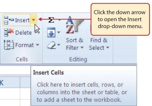
MedAttrib: Beginning to Intermediate Excel. MS Excel Insert Button (Down Arrow).

•  Click cell C1.
• Click the down arrow on the Insert button in the Home tab of the ribbon.
• Click the Insert Sheet Columns option from the drop-down menu. A blank column will be inserted to the left of Column C. The contents that were previously in Column C now appear in Column D. Note that columns are always inserted to the left of the activated cell.

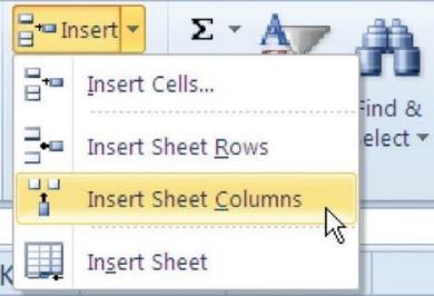
MedAttrib: Beginning to Intermediate Excel. MS Excel Insert Drop-Down Menu.

• SAVE your work, and close the file. EXCEL ACTIVITY #1 FINISHED.

Worksheet Formatting and Inserts

Worksheets have a lot that can be done to them alone. They are part of a bigger workbook (and sometimes one worksheet makes up the whole of a workbook. In this segment we’ll cover the manual formatting and steps you can do on a worksheet.

• First, let’s consider the worksheet item. Near the bottom of a worksheet, a small tab will have a name on it; by default this would be Sheet1, Sheet 2, etc. Double clicking on the name activates the name field so you can change the sheet name.

TIP. Sheet names. You should always assign a clear and simple name to a worksheet that designates what it is for. Later, when looking at formulas for data management, simple named sheets are much easier to keep track of when building formulas.

Managing sheets

Next to the worksheet tab Excel offers a Plus sign, which allows the quick addition of new worksheets under their default name convention.

• Right-clicking on the sheet name shows a context menu that allows you to add or delete sheets, copy and move sheets, protect sheets, add a tab color, and select multiple sheets to group.

Sheet data formatting

Worksheets, like documents in MS Word, offer many text formatting options. Other than differences in text strings and numeric calculation data in cells, all the content in a worksheet can be formatted to look different:

Home tab – Clipboard Group

At the very left of the Ribbon is the clipboard group, which is a small set of tools you can use in relation to when text, images, and styles have been saved to the clipboard as you work. Clipboard-related activities include:

• Copy
• Cut
• Paste
• Redo
• Undo
• Paintbrush
• Moving info by dragging

Format Painter – Home tab clipboard group

• Allows you to “capture” an existing style and apply it to any object you click on.
• Single-click applies once
• Double-click locks so you can reuse it

Understanding the clipboard

• See the Clipboard Pane by clicking Home tab/Clipboard section expander icon
• Can “store” numerous pieces of text and images
• Items are stored temporarily (in RAM) until the program is closed.
• You can also delete items off the clipboard.
• You can store them and then choose which one to paste

Home tab – Font group

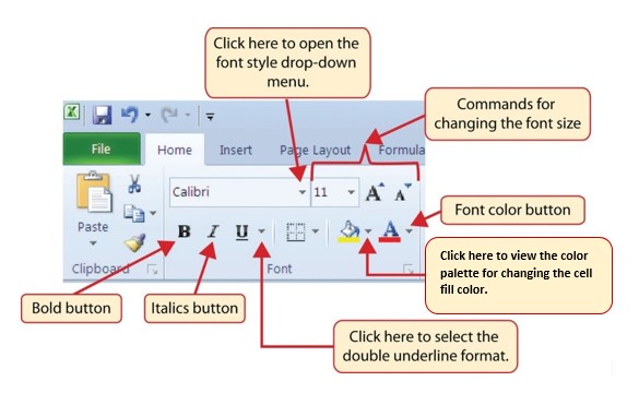
MedAttrib: Beginning to Intermediate Excel. MS Excel Home tab Fonts group.

“Fonts” refer to the letters (characters) used in text. Font formatting includes resizing, changing the font family, adding bold or emphasis, adjusting spacing between letters, and more. You can right-click on a word or cluster of words for the contextual menu, or use the Home Tab’s font group options. These include:

• Style (font family)
• Size
• Color
• Bold, italics, underlining, strike-through
• Changing text size
• In Excel, the font color and cell background color (paint bucket) are also in the Font group.

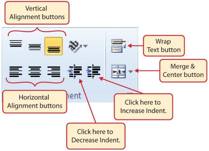
Home tab – Alignment group

In Excel, alignment means the placement of text inside a cell. The data you input into cells, unless formatted into some numeric form, defaults to a Bottom Alignment and to an Align Left. Any workbooks you inherit may change these defaults, and you may develop a preference.

MedAttrib: Beginning to Intermediate Excel. MS Excel Home tab Alignment group.

Home tab – Number group

Text is easy to work with in Excel – the program just recognizes it as static data that is informational, not computational. However, numbers (unless used in something like an address or phone number) are recognized as data to calculate.

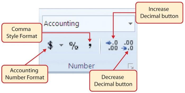
MedAttrib: Beginning to Intermediate Excel. MS Excel Home tab Number group.

There are several types of numeric data that Excel recognizes, including:

• Comma, which adds a comma and a decimal point with a default 2 decimals after the decimal point.
• Dates, which offers both long and short US date formats
• Time
• Percentage
• Currency (explained below)
• Accounting money (explained below)
• Fraction

Text Formatting

The following steps demonstrate several fundamental formatting skills that will be applied to the workbook that we are developing for this chapter. The basic worksheet formatting tasks can all be found on Excel’s Home Menu Ribbon in the Font group.

ACTION: MS Excel Try Me Activity #2

This activity is a modification from MS Excel BootCamp.

Let’s do a few basic Excel text formatting tasks. Let’s use the Excel_formatting.xlsx file that should be in your DataFiles folder.

Before you start, you should use your file manager utility to make a copy of the Excel_formatting.docx file that is in your DataFiles folder, then paste the copy into your Examples / MS_Excel folder.

Here is an example of what we are aiming for from the starter file you are working with:

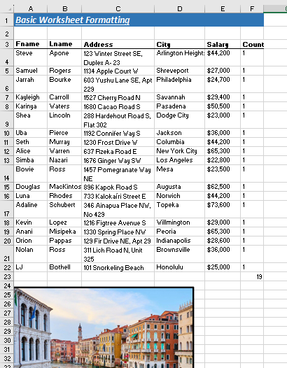
MedAttrib: author-generated. MS Excel example formatting file.

• If Excel isn’t open yet, open MS Excel.
• Open a file, and use the browser dialog panel for the Excel_formatting.docx file that should be in your Examples / MS_Excel folder, then open it.

The Home ribbon has 9 groups. In this series of tasks, we’ll work with the Clipboard, Font, Alignment, and Styles groups.

MedAttrib: Beginning to Intermediate Excel. MS Excel Font Group of Commands.

Text Size and Styles

First, we’ll work on Row 1, which is a document identifier title.

• Select cell A1. You can see it is selected in the formula bar and is active.
• With the cell active, choose the Text size in the Font group and select 18. This makes the text a larger 18pt size.
• Then, from the Font group, click the buttons for Bold, then Italic, then Underline.

Keyboard Shortcut: Text Formats. Hold down the CTRL key while pressing the letter B (Bold), or I (Italic) or U (Underline) on your keyboard. MAC Users: CMD key.

Cell and Text Colors

You can emphasize a region of a spreadsheet by adding color to the cells and/or text.

• Select the cells A1-F1. You may see the contents of only A1 in the formula bar, but also a selection outline around the 6 cells you chose.
• Find the paintbucket Fill Color button on the ribbon’s Font group, and click the down arrow on its right side. This will show you a color palette to choose a cell color from.
• If you hover over the colors, a tooltip will appear with the color’s information. Click on Blue, Accent 5 Darker 25%, which is the second to the last column of colors, and second from the bottom of that column.
• Click only cell A1 again. Then using the Font Color button on the ribbon’s Font group, click the down arrow on its right side. This will show you a color palette to choose a text color from. Select White.

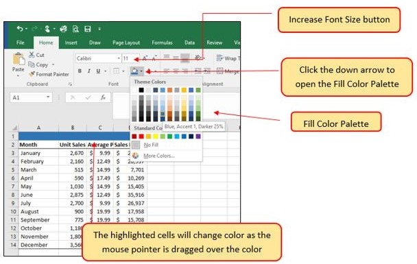
MedAttrib: Beginning to Intermediate Excel. MS Excel Fill Color Palette.

Merge Cells

Data is entered solely into one cell at a time, like the exercise example’s rows and columns. However, for stylistic purposes, data can also be merged into more than one cell. For instance, the Merge & Center command is used to center the title of a worksheet directly above the columns of data.

• Select cells A1-F1 again.
• Click the arrow on the Merge & Center button in the Font section of the Home ribbon to select the Merge and Center setting.

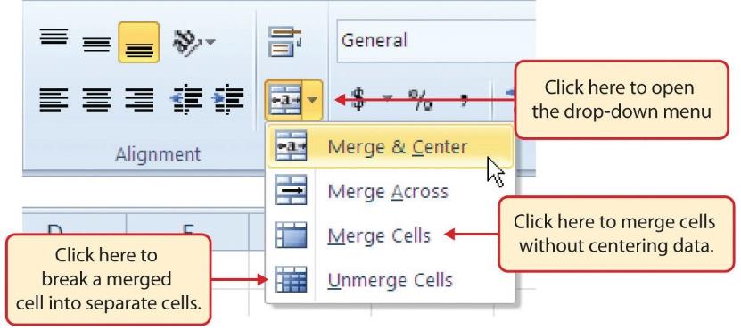
MedAttrib: Beginning to Intermediate Excel. MS Excel Merge Cell Drop-Down Menu.

• SAVE your work.

Header rows

Any range of data in Excel that you may want to sort, filter, and/or calculate should have a Header Row, which is a row that you use to identify the expected contents of the columns of data. Sometimes you may see instead a header column, but for this course the norm will be the header row above columns.

The header row should stand out from the rest of the range of data for ease of identification.

• Select Cells A3-F3
• Using the technique above, make them Bold.
• With the A3-F3 cells still active, click the ribbon’s Font group Border button’s arrow on the ribbon and select Bottom Border.

Borders

In Excel, adding custom lines to a worksheet is known as adding borders. Borders are different from the grid lines that appear on a worksheet and that define the perimeter of the cell locations. The Borders command lets you add a variety of line styles to a worksheet that can make reading the worksheet much easier. The following steps illustrate methods for adding preset borders and custom borders to a worksheet:

• Click the down arrow to the right of the Borders button in the Font group of commands in the Home page of the ribbon to view border options. (see Figure 1.40).
• SAVE your work.

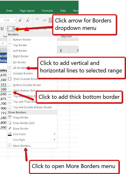
MedAttrib: Beginning to Intermediate Excel. MS Excel Borders Dropdown Menu.

Autowidth Expansion

You may find that the column E for the salary data is showing pound signs (####) in the data cells. This indicates that a numeric column is too narrow to accommodate the data in it. Whie a text column will show some of the data in a too-narrow column (like the Address column noted above did), Excel can’t do this with numbers, and Excel can’t do wrap text for numeric data either, because numeric formats are for calculations, not static information.

You can fix this issue by widening the column. We’ll cover more column-related sizing later, but for now, the Autowidth action will suffice.

• Select the whole column E – by clicking on the E column’s address E at its top. Your cursor tip should then show a down arrow.
• Slowly move your cursor to the right until the tip shows a Crosshair graphic. This means you have hovered over the border between columns E and F.
• Double-click while you see this crosshair, and column E should snap to a width that shows all the numbers within.

Alignment of Cell Content

The data you input into cells, unless formatted into some numeric form, defaults to a Bottom Alignment and to an Align Left. Any workbooks you inherit may change these defaults, and you may develop a preference. For this worksheet, we’ll go for Top Alignment and Align Left. The file we are working with currently shows the first two columns are align center.

• Select cell A3, and click the Top Align button on the ribbon’s Alignment section.
• With A3 still selected, then click the Align Left button.

MedAttrib: Beginning to Intermediate Excel. MS Excel Alignment Group in Home Tab.

You can change the alignments of several cells at one time:

• Select cells A4-A21.
• Click the Top Align and Align Left buttons again. The rest of the column should now look like Cell A3.
• Now, select cells B4-F21, and click the Top Align and Align Left buttons again. The rest of the table will also be top aligned and aligned left.

There is just one cell may remain unaligned properly: cell B3. Let’s use the Excel Format Painter button to fix that. The Format Painter button will pick up the formatting of a cell, and hold it until you click on another cell to ‘copy’ the format onto it.

• Select cell A3.
• Click once on the Format Painter ‘paintbrush’ button in the Home ribbon’s Clipboard group.
• Then, click on cell B3. This should copy cell A3’s alignment format onto cell B3.
• SAVE your work.

Wrap Text

Often, a column may have not be wide enough for the information in it, and the data will seem to be cut off. One way to fix this is to wrap text so that the cell will increase in size to accommodate the data.

• Select cell C4.
• Click on the Wrap Text button in the Home ribbon’s Font group. See how the row expands in height to show all the data.
• Now, while cell C4 is still active, click on the Format Painter button from the Clipboard group.
• Then, while the Format Painter is active, hover and click over cells C5-C21 to apply the wrap text to the rest of the column.

Keyboard Shortcut: Wrap Text. Press the ALT key and then the letters H and W one at a time. MAC Users: n/a.

Number Formatting

Text is easy to work with in Excel – the program just recognizes it as static data that is informational, not computational. However, numbers (unless used in something like an address or phone number) are recognized as data to calculate. There are several types of numeric data that Excel recognizes, including:

• Comma, which adds a comma and a decimal point with a default 2 decimals after the decimal point.
• Dates, which offers both long and short US date formats
• Time
• Percentage
• Currency
• Accounting money
• Fraction

For this example, let’s first format the Salary columns contents with a comma so that the numbers look like common ‘thousand’ units.

• Select cell E4.
• Look for the Home ribbon’s group called Number, and the dialog box arrow, which will show a dropdown selection of number formats. Click that button.
• Scroll down that list until you find Currency, and click on that. The cell’s contents will now appear as $44,200.00.
• Let’s take out the “cents” part of that number. With cell E4 still active, click twice on the Number group’s Decrease Decimal. This should remove the .00 from the number.
• You can repeat the Currency format and Decrease Decimal steps after you select cells E5-E21.
  • Alternative method: use the Format Painter paintbrush to paint Cell E4’s format over cells E5-E21. Click once on the Format Painter ‘paintbrush’ button in the Home ribbon’s Clipboard group while cell E4 is active, then paint over cells E5-E21.
• SAVE your work.

MedAttrib: Beginning to Intermediate Excel. MS Excel Number Group of Commands.

The Format Cells Panel

• When you become proficient with Excel and the content you plan to produce, you can also use a more comprehensive Format Cells panel, which has several tabs you can choose from while formatting a cell or row or column.

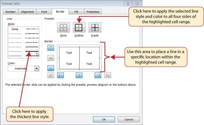
MedAttrib: Beginning to Intermediate Excel. MS Excel Borders Tab of Format Cells Dialog.

Here, we will add a line to the bottom of the data range we have been working on, so that you can input some data yourself, then format it.

• Click on cell A22, and type YOUR own first name in it.
• Add more information for yourself in cells B22-F22. Other than your own real last name, please feel comfortable ‘making up’ data for the other cells so that you preserve your confidentiality.
• Once you have your new data entered, click on cell A22.
• Then, in the Font group on the Home ribbon, look for a tiny Font settings arrow icon in the group’s lower right corner, and click on it. This should open the panel for Cell Formatting, which has 6 tabs in it: Number, Font, Alignment, Border, Fill, Protection.
• Since Cell A22 is a static text data, you can use the Font and Alignment tabs to look at your choices and to change the cell’s format.
• Using the Alignment tab, make the contents of cell A22 top aligned, left aligned if it is not already, then click Okay.
• RIGHT-Click on cell B22, then scroll down the contextual menu until you see the Format Cells option (you may have to scroll down the menu list since it is near the bottom). Then, click on the Format Cells option. The same Cell Formatting panel you have already used will open.
• Using the Alignment tab, make the contents of cell B22 top aligned, left aligned if it is not already, then click Okay.
• Now, you can use either of these options to open the Cell Formatting panel as you adjust the formats of cells C22-F22.
• OR, you can just select cells C21-F21 and click the Format Painter paintbrush button on the ribbon, and then run the style over cells C22-F22.
• SAVE your work.

Special Formatting

Much of your data formatting will be basic tasks, like changing the color of the text or cell backgrounds, cell/column/row alignments and wrap, and selecting basic numeric formats like dates, accounting, percentages, etc. However, there are a number of basic additional formats that Excel lets you customize for more complicated needs, like:

• Phone numbers
• Social Security numbers
• Zip codes
• Showing negative numbers in stand-out formatting
• Additional date and time formats
• Additional fraction formats
• Customized number formats
• Validation techniques

These options are shown in the Format Cells panel, in the Number tab.

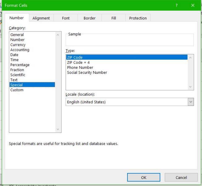
MedAttrib: autogenerated. MS Excel Format Cells panel.

Examples:

• Phone number: 2065551234 = (206) 555-1234
• Social Security Number: 2221111234 = 222-111-1234
• Zip Code + 4: 981012345 = 98101-2345
• Negative Number (one of the formats): -2700 = (2,700)

AutoSum feature

Applying mathematical computations to a range of cells is accomplished through functions in Excel. However, the following steps will demonstrate how you can quickly sum the values in a column of data using the AutoSum command in the Home menu ribbon:

• Click cell F23 in the worksheet.
• In the Home tab’s ribbon, look for the Editing group (more to the right of the ribbon).
• Look for the button that looks like an and reads Sum when you hover over it. Click it while cell F23 is active.

What you’ll ‘see’: Cell F23 will turn into a formula – =SUM(E4:E22) – and a dotted border and light blue fill will affect the column of numbers above it.

• When you press the ENTER key on your keyboard, the sum will calculate automatically, and add up the numbers in the column above cell F23.

Now you will see the number of people in the data range we have been working with, including the row you input about YOU!

• SAVE your work.

Inserts

In Excel, graphics like images, icons, and shapes We won’t cover all the insert options, but they work much the same way as the Picture one.

Excel lets you add illustrations, like photos, clipart, WordArt, SmartArt, icons, and shapes. Inserts are ‘unanchored’ to cells, which means that they float above cells and can be easily moved without affecting the data typed and calculated inside your cells. Like in Word, in Excel an inserted item like a picture – when made active by clicking on it – will reveal a contextual Menu ribbon for doing editing work on the inserted item.

• With the Excel_formatting.docx file still open, let’s insert a picture.
• Place your cursor around Cell A25.
• In the Inserts menu ribbon, click the Illustrations group button for Pictures.
• Click Pictures, which shows you image locations to choose from: This Device, or Stock Images, or Online Pictures.
• In this case, assuming you are online, choose the Online Pictures option, which will pull open an Online Pictures window only.
• Then, type in the name of your favorite place – if you have one – and look at the results you get. Then, choose one and click it, which will insert it into your worksheet.

Your image could be in any size, so we’ll set a size for whatever image we use to practice resizing.

• Click your inserted picture. This ‘activates’ the picture so that a new, contextual menu/ribbon appears at the right-hand side of your Menu bar, called Picture Format. We will use this ribbon for the next several steps.
• In the Picture Format ribbon, on the far right, choose the text field for the horizontal size, and type in 3”. This will resize your picture to 3 inches wide, and to whatever the proportional height is.
• Next, click the Accessibility button on the Accessibility group. In the text field, type “image of my favorite place (and the place’s name)”, and place a checkmark in the Mark as decorative checkbox. This allows Excel to consider this image as accessible in the program.
• Then, in the Picture Styles group, choose Picture Border, and in the dropdown, choose the color black. This adds a very narrow border to your picture.
• in the Picture Styles group, choose Picture Border again, and in the dropdown, choose Weight, and on the flyout menu, choose 3pt. This will make a more prominent border for your picture.
• SAVE your work, and close the file. EXCEL ACTIVITY #2 FINISHED.

Workbook Design

Workbooks are made up of one or more worksheets, and are like a book holding file folders. Each worksheet can contain different data, but be part of the same project. You will likely – in the workplace – inherit existing workbooks, or create your own with multiple worksheets (pages). Managing them in the workbook, and designing the workbook itself, is a useful skill.

ACTION: MS Excel Try Me Activity #3

This activity is a modification from MS Excel BootCamp.

For this chapter, we will use the data file Excel_design.xlsx in order to demonstrate the various steps. Please find and open Excel_design.xlsx, and save a copy to your Examples folder. Most of our work will use the Page Layout menu ribbon for themes, colors, fonts, and effects.

Adding and Deleting Worksheets

Now, let’s add, then delete, new worksheets in this same file (workbook).

• The Excel_design.xlsx file currently has one worksheet, named Sheet1. Click anywhere in the worksheet.
• In the worksheet’s name tab section, double-click name tab that reads Sheet1. You can overwrite that name; rename the sheet Desserts.
• In the worksheet’s name tab section, click the + to add another worksheet tab, which will default name itself Sheet2. It will appear just to the right of Desserts.
• Click the + to add a third worksheet tab, which will default name itself Sheet3 and appear to the right of Sheet 2.
• Click the + to add a fourth worksheet tab, which will default name itself Sheet4 and appear to the right of Sheet 3.

We actually do not need all of these sheets.

• Choose Sheet2, so that you are in that blank sheet, then look in Home menu ribbon for the Cell group.
• Click the down arrow on the Delete button and choose the Delete Sheet option from the drop-down list. This removes the Sheet2 worksheet.
• Click the Delete button on the Delete warning box (if a warning box appears).
  • Alternate method: RIGHT-click on the tab of Sheet3, which will offer a contextual menu. On the menu, click Delete.
• SAVE your work.

Keyboard Shortcut: Inserting New Worksheets. Press the SHIFT key and then the F11 key on your keyboard.

Renaming worksheets

The default names for new worksheet tabs at the bottom of any workbook are Sheet1, Sheet2, and so on. However, you can change the worksheet tab names to identify the data you are using in a workbook. Additionally, using you can change the order in which the worksheet tabs appear in the workbook, and using that same process add a worksheet, delete one, protect one, etc.

The following steps explain how to rename and manage the worksheets in a workbook:

• Double-click the Sheet4 worksheet tab at the bottom of the workbook. Type the name Beverages.
• Press the ENTER key on your keyboard. Now we have a nice, empty sheet.
• Moving worksheets

There are a couple of ways you can move a worksheet. We’ll try both for practice.

• Right-click on the Beverages worksheet’s tab name. In the dropdown menu, select Move or Copy from the dropdown menu.
• In the Move or Copy panel, do NOT put a checkmark in the Create a copy checkbox. This is so that the Beverages sheet will only be moved.

The To book field will show the name of the current file, since we are moving inside the same file.

• Then, in the Before sheet, click Desserts (to move before that sheet) and click the OK button. The Beverages sheet should now be the first available worksheet tab at the left.

TIP: Copying/moving worksheets. You can use this same technique to copy a worksheet to add somewhere in the same workbook, or to start another workbook altogether. You would make sure to put a checkmark in the Create a copy checkbox. To open the copy to a new workbook, you would also choose to move to (new book).

Nope, we don’t like it there. Let’s move it back.

• Press your mouse cursor down on the Beverages worksheet’s name tab, until you see a small icon of a sheet of paper floating near your cursor. That is the indicator that you can, while still pressing down on the mouse cursor, drag the worksheet tab.
• Drag the Beverages worksheet tab to the right of the Desserts worksheet tab, then release the mouse/cursor. The Beverages sheet should now be at the end of the row of worksheet name tabs.
• SAVE your work.

MedAttrib: author-generated. MS Excel worksheet design final result.

Page Layouts – Page Layout Tab

In MS Word, documents allow both a design and layout Menu ribbon. Because Excel is mostly about analysis and calculation, the essential design and layout options have been combined into the Excel Page Layout menu/ribbon. The Page Layout tab allows you to set the physical format of your worksheet. What you do here will stick with your document and once in the Print preview before printing/distributing your work, the prepared output should be assured.

Setting up documents – Page Layout tab

The Page Layout tab allows you to set the physical format of your page, which is a good starting step in word processing work. This determines how large the paper used will be, the margins, the orientation of the document, etc. In the Layout tab’s ribbon, you can use the page setup group icon dropdowns, or the group’s panel activation arrow, to accomplish (in order of page setup group).

TIP: Multiple Worksheet set-up: You can select all the worksheets in your workbook and set the Page Layout options all at once, if you know what your project parameters will be.

• Page margins: the white space around the edges of a page that won’t be printed on , and also which adds white space around a document’s content for viewability.
• Page orientation: the height and width direction of a page. Default and common use is Portrait, in which a document is taller than wide. Horizontal is commonly more useful in Excel since ranges of data/tables can be wide, with many columns.
• Page size: the paper size of a document, even if it never is intended to be printed on paper. Users may choose to print the document, print a PDF, and or take a screenshot image for later printing/pasting into another document. The default is 8.5 x 11 inches, with other common page sizes being legal (8.5 x 14 inches), and ledger (11 x 14inches). Other listed sizes may be legacy for office documents. In Excel, a common selectin is 8.5 x 14, since tables with many columns of data tend to be wide.
• Breaks: You can create a new page break, a break to begin and end a different column style, or wrap text around an inserted image, and add new section breaks.
• Print area: This allows you to designate a specific range of columns and rows to be printed, even if it is smaller than the whole of your worksheet’s contents.

For this workbook, Excel_design.xlsx, let’s adjust the layout of the margins, page orientation, and page size.

• Click anywhere in the Desserts worksheet.
• Go to the Page Layout ribbon’s Page Setup group, and click Margins.
• With Margins open, choose Narrow. Then, click Margins again, and choose Custom Margins (at the bottom).

Custom Margins will open the Page Setup panel, and the Margins tab in it. Make the changes to the margins that you see in the image below:

• Top margin=1, Bottom margin=.70, Header=.25, Footer=.25, Center on page=Horizontally

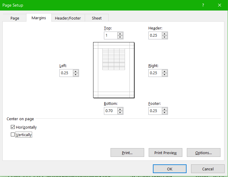
MedAttrib: author-generated. MS Excel Page setup.

• Click OK to exit the Page Setup panel.
• Next, choose Orientation from the Page Layout ribbon’s Page Setup group.
• Choose Landscape. The default is Portrait, which makes the worksheet print-out taller than it is wide. Landscape will make it wider than tall, and help accommodate more columns of information on the same page.
• Now, choose Size from the Page Layout ribbon’s Page Setup group.
• In the Size dropdown, choose Legal. Legal is often used for spreadsheets due to their many columns that need to appear on a single page.
• SAVE your work.

Designing documents – Design tab

Themes apply decorative styles to your Excel worksheet, such as fonts, colors, effect options, paragraph spacing, etc. They can give a set of documents a consistent and attractive appearance and make your word processing efforts look more professional. In business, they are best used as part of a “package” of documents, such as a letterhead and envelope set or as part of a report style. They can enhance what you want to communicate by adding company branding colors and fonts. You can also:

• Make your document more readable than just black-and-white text.
• Tie consistent inserts, like shapes and borders, together with the rest of the document’s “look”.
• Use different colors and font styles to punctuate header rows from the data cells.
• Easily update the whole look of your document just by changing the color or font variants
• Design: Theming / Design Tips

Using themes can be a double-edged sword. While they can add attractiveness to your documents, they can also, if misused, make your work look confusing, be hard to read, and muddy your communication message.

• Choose theme colors that make sense for the product, service, or idea(s) you are trying to communicate
• Choose theme backgrounds that have good contrast and allow text to be very easy to read
• Choose fonts for readability, based on need for headlines, lots of paragraph texts, easy bulleting, etc.
• Remember that less is more – more colors and font variations in one document can look unprofessional and take away from your message.

Design: Theme Variants

Theme variants let you change aspects of a theme you select to apply a different core font family to it, or to change the color palette it will work with.

• Fonts: Font families in themes are designed and sized to be readable and hopefully scannable by screen readers for accessibility use. The style will offer a font for titles/subtitles, and another for general text. Available font families come installed with the computer’s operating system, and may also be accessed from the word processing software’s installation or cloud-based accessories.
• Color Palettes: Like fonts, color palettes are included in a style, and can also be changed independently to modify and create a new style. For instance, the overall design style of a theme may work for you, but the color palette assigned to it may not have enough contrast for your audience, or your company may focus on a different rage of core colors.
• Effects: These are subtle styles that can be attached to some inserted items, like image borders, shapes, SmartArt, etc.
• Scale to fit group: Scale to fit in Excel is a way to preset your worksheet for print views.
• Sheet options group: This group lets you designate if you want to see gridlines on your sheet while you work. Grid lines are not the same as borders, and will not appear on printed pages.

Using Themes

We’ll start with the Page Layout ribbon. This is because when putting together a spreadsheet, it is efficient to work from the macro level to the granular level; the theme, colors, and other things that affect all the styling of the worksheet should be considered when creating the project, so that any inserts, tables, and charts/graphs flow from the color and font selections.

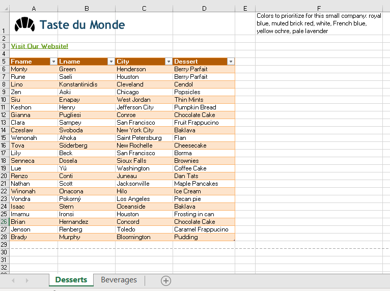
In Excel_design.xlsx, we’ll change the theme first, then determine if it meets our needs and how to adjust it by choosing other colors and/or fonts. Normally, Excel defaults to the current Office theme, which gives a palette of colors and shades from across the color spectrum. However, on spreadsheets, you may instead prefer a different color set, or inherit a workbook at work that uses another color scheme, or be tasked with an assignment with certain theme specifications. While Excel is designed for themes to be changed almost effortlessly and without technical glitching. It is always good to plan your work and do steps efficiently to avoid rework or conflicts to very large spreadsheets later.

Colors to prioritize for this small company: royal blue, muted brick red, white, French blue, yellow ochre, pale lavender. We’ll find out what applies in the color themes, if any. Blues and related muted colors are preferred.

• Click on cell A1, then choose the Page Layout menu ribbon.
• In the Themes group of the ribbon, choose the Themes dropdown box arrow.
• For fun, just click on a few – on your screen outside the Themes dropdown, you can see the fonts, header row color, and the Taste du Monde “croissant” image effects seem to Preview a change.

We’ll settle on the Berlin theme, because the font selection seems easy enough to read with a little added text boldness, but not too stylistic to make a workbook hard to understand.

• SAVE your work.

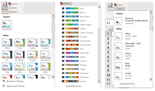
MedAttrib: author-generated. MS Excel themes/colors/fonts dropdowns.

Modifying Themes

Now, the Berlin theme has great fonts, but the color palette may not work. Let’s check it out. The Taste du Monde header row is currently kind of an orange-brown color. Not good for the company’s planned color scheme.

• Right-click on the cell A5, the first cell in the header row, which will pull up a menu list.
• Choose the Format Cells (you may have to scroll down the menu list since it is near the bottom), which opens the Format Cells panel. In this panel, choose the Fill tab.
• In the Fill tab, look at the upper left that shows a palette of 10 columns of colors and their shades. This is the color palette for this particular theme, and includes maybe a couple of the muted French county colors we could use, but no blues. No thank you!
• Exit the Format Cells panel by clicking Cancel.

Colors Palette

Now, let’s consider other color options for this theme. While keeping the Berlin theme, we will use the Colors panel to look at options and change the color palette.

• You can click anywhere on the work area of your worksheet; then In the Themes group of the ribbon, choose the Colors dropdown box arrow.
• We are looking for something that has a dark blue, medium blue, darkish brick red, and a couple of neutral colors in the palette that could be purposed for Taste du Monde. Scroll down the Colors dropdown, and notice how our header row’s color changes. The closest we may find is the Aspect color palette.
  • Note: this course is focusing on Excel for Windows (PC) and the assumption that your full installation has all the built-in items, like themes, color palettes, etc. However. If you don’t have some of these themes or named palettes / font collections, choose what you can to gain the skills-building anyway.
• In the Colors palette, choose Aspect (near or at the bottom of the list). This looks mostly like reds and so we’ll repeat looking at cell A5 in the Cell Format panel’s Fill Tab to check out the color palette’s spread of colors.
• In the Cell Format panel’s Fill Tab, look at the color palette. In it, there is a blue column with a dark blue and a French blue, dark brick reddish color, a lavender color, a kind of light tan, and white. This should do. We can use a later use a color search for a pale yellow, if needed.
• Click on the 7^th column’s dark blue (second from the bottom), which will fill the A5 cell, then click OK.
• Use the Home menu’s Format Painter paintbrush to paint the style of cell A5 over B5-D5.

Fonts Palette

Because the Taste du Monde’s header row had already had a dark color, the text was already white, so we do not need to change the text color for readability / contrast. However. We can look at the Fonts palette to determine if we want a different font set.

• You can click anywhere on the work area of your worksheet; then In the Themes group of the ribbon, choose the Fonts dropdown box arrow.
• In the dropdown list, there are a number of font sets. Unfortunately, the dropdown list does not show which specific font set we are using. You need to click on one of the cells in your workspace to see, in the Home ribbon’s Font Field which font this document is using: Trebuchet.
• Scroll down and see how the fonts on your worksheet seem affected in the preview. You can choose to experiment by clicking on one or two, but for Taste du Monde, we’ll stay with the Berlin theme’s chosen fonts.
• SAVE your work.

Effects Panel

The Effects panel lets you preview some effects that can be used on graphics like shapes, SmartArt, WordArt, and image borders in Excel workbooks. In this Taste du Monde worksheet, there is already a croissant image that we can use to observe what happens with effect changes.

• In the Themes group of the ribbon, choose the Effects dropdown box arrow.
• For fun, just click on a few – on your screen outside the Effects dropdown, you can observe the croissant image effects in a Preview. Some of the effect options seem to make a big change; others seem barely noticeable.
• Click on the Frosted Glass effect to choose it.
• SAVE your work, and close the file. EXCEL ACTIVITY #3 FINISHED.

Now you should have a good handle on basic workbooks design.

Datasets

Excel is all about data. The data is for viewing, organizing, sorting/filtering, analyzing, and calculating so that business problems can be considered and solved. The more organized the data is, the better you will be able to use it, analyze it, and get the needed calculations, graphs, and pivot tables to answer your questions.

A dataset is simply a range of data – a range of cells in tabular format. It may be formatted or unformatted, have an assigned name or be in a table object.

ACTION: Quick Task

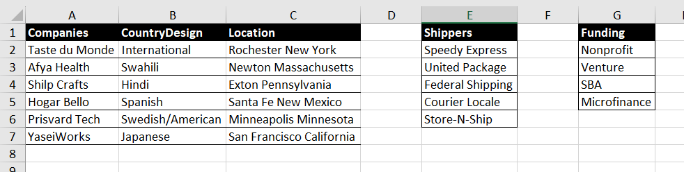
Let’s look at an image of some Excel work. In it the cells A1 through D7 have data that seems related to each other. Cells E1-E6 is a column of data, as is the column of G1-G5. This is all part of a dataset, although only cells A1 through D7 seem to meet the dataset definition of being contiguous.

MedAttrib: author-generated. MS Excel dataset.

Understanding Cells

• Cell contents: As discussed above, all data in Excel (other than inserted objects like pictures) is input into cells. Each cell is something that, as part of a row and column, can be sorted, calculated, and tell a story.
• Cell addresses: Data are entered and managed in cells by entering numeric and non-numeric data. Each cell in an Excel worksheet contains an identification address, which is defined by a column letter followed by a row number. For example, the top left cell A1. This would be referred to as cell location A1 (or cell reference A1). You can navigate in an Excel worksheet with your mouse pointer or using the arrow buttons on your keyboard.
• Column Headings: In Excel, data rarely means anything to a viewer if there is no context attached to it. Commonly this is done through column headings, which identify what the content in the column is supposed to be. This can also be done as row headers instead, but in this course we’ll mostly use the standard column headings.

Rows/Columns

Rows and columns can be adjusted to help make visualizing and analyzing data easier.

• Resizing: You can resize columns from the Home tab Cells group to reveal information that looks cut off, or to narrow them if there is too much space. Same with rows if the row is too tall or seems to have cut off anything other than the first line of text.
• Inserting/Deleting: Rows and columns can be inserted as needed from the Home tab Cells group, in order to expand for data to be added. Existing columns and rows can also be deleted.
• Hiding/Unhiding: You may have a worksheet with a lot of columns, but really only need to see some of the data to analyze/decide on an action. Hiding columns or rows can help you focus.
• Sorts: In addition, information in a dataset can be sorted from the Data tab Sorts & Filters group, so that a column shows information in an alphanumeric order or in some more customized order.
• Filters: A dataset may have information about more customers or other content than you need: using a filter from the Data tab Sorts & Filters group lets you temporarily hide unwanted information so you can get a snapshot view.
• Freezing Panes: If a dataset is made up of hundreds of record – long enough that you need to scroll down several pages to see it all, or over enough columns that you can’t see the important left-most columns, you can freeze a column or two, or the header row, so that the information remains in view no matter how much you have to scroll.

ACTION: Quick Task

Back to the image again:

MedAttrib: author-generated. MS Excel dataset.

In here, all three batches of data are ‘ranges’ of data. This is important, because we may want to actually reference them in a tidy way for formulas and general reference. As they exist now, they are simply designated by the cell collections. A1:C7, E1-E6, G1-G5.

Conditional Formatting – Home Tab

You can apply conditional formatting based on specific conditions you want to be highlighted. Example: contents of cell is less than a certain quantity.

Data – Data Tab

Excel allows you to manipulate data – how it is sorted, imported, filtered, validated, and grouped.

• You can import existing data from the web, another spreadsheet, a database, XML, and more (advanced).
• You can sort rows and columns, such as for alphabetizing.
• You can filter tables to show only certain rows or tables based on criteria you set – the rest is simply hidden, not gone.
• You can remove duplicates of data.
• You can group info to create subtotals, before totaling those.
• You can use flash-fill to add large amounts of consecutive data.

As noted above, a dataset is simply a range of data. However, what needs to happen with data is what is important. Formulas that calculate data for specific purposes need to be able to find the data and easily add it to the formula. Sometimes the data will be all the contents of a table. Sometimes it will be only a column or two, or a few rows. In these cases, being able to “set aside” the data range in an identifiable way is crucial. You can do this by identifying data ranges.

• Selecting: You select a data range by choosing a selection of row and column cells, such as A1 through D10, or A1:D10.
• Naming: To make that data range useful and easy to refer to in a formula, you need to name it. This can be done in the Formulas tab’s Defined Names group by using the Name Manager panel to give the data range a name. Once this is done, you can see a list of every named data range in the Excel Address field.
• Use in formulas: In a formula, you can use the named range as the data range reference in the formula.

ACTION: MS Excel Try Me Activity #4

This activity is a modification from MS Excel BootCamp.

Let’s now work with an Excel file: Excel_datasets.xlsx. This is a dataset from our friend Taste du Monde that we can use for looking at a dataset, identify ranges of data, and set names for two or three of them.

Save a copy of Excel_datasets.xlsx to your Examples / MS_Excel folder, then open it for work. It already includes the Taste du Monde logo icon and WordArt and link to their website. It also includes records of customer data including names, addresses, emails, and opt-in decisions.

The whole set of A6 through J36 is a data set.

• Select only cells A6 through C36. This is a range of data of that range of cells of customer names and their customer ID.
• Deselect it.
• Select only cells A6 through J9. This is a range of data of the first two customer records.
• Deselect it.

Now, let’s choose a range of data and name it for possible later use.

• Select only cells F6 through H36.
• With these cells selected, choose the Formulas menu ribbon.
• In the Formulas ribbon, look at the Defined names group. Select the dropdown arrow of the Defined Name button.
• Click on “Defined name”, which will open a dialog box.
• In the dialog box, in the Name field, type TM_Region.
• In the dialog’s Scope, leave the default of workbook.
• In the comment field, type: Taste du Monde customer regions.

In the Refers to field, note that Excel recognizes that you selected as =Customers!$F$6:$H$36, which is referring to the worksheet called Customers, and the range of data from F6 through H36. Click OK.

• Now, click on the dropdown arrow of the Name box in the Excel UI, which usually shows the address of the Cell you have clicked in. When you click on the arrow, you should see TM_Regions listed. This is a named data range.
• Click on TM_Regions in the Name box. Excel will select the range of data you just named – cells F6 through H36.
• SAVE your work.

Moving ranges

Let’s move a named range.

If you have not yet saved Excel_datasets.xlsx, DO IT NOW, please. We will do a task we may not want to keep but you don’t want to lose any previous work.

• With Excel_datasets.xlsx still open, use the Name box to choose TM_Regions. Excel will select the cells that make up that named range.
• Right-click and choose Cut (or use the shortcut of CTRL X / CMD X for Mac), which will ‘cut’ the selection.
• Place your cursor in cell L6, right-click, and choose Paste (or CTRL V / CMD V).

The named range has been moved.

• Close the Excel_datasets.xlsx without saving it.

Sorting data

Let’s work with sorting and filtering data ranges. We actually want to work with the Excel_datasets.xlsx file again. We just didn’t want to save the last set of changes made. Please open the Excel_datasets.xlsx file.

The dataset has a header row, which has been emphasized with bold text. This will help us identify what we want to sort and filter.

The important thing to know about datasets and named data ranges is that, although they display data in columns and rows, the data is not actually connected. Let’s see what this means.

• Select the contents of Column I, Cells I6-I36. Copy it, then move your cursor to Cell J6.
• In Cell J6, paste the data you just copied. Now you have two columns of Opt-In responses.
• Select the data of Column J: Cells J6-J36. Use the format painter in the Home ribbon to paint the cell backgrounds a light color, like gray.
• With this J column data still selected, choose the Data ribbon. In the ribbon, choose the Sort & Filter group, Sort A to Z button.

You should see a sort warning message:

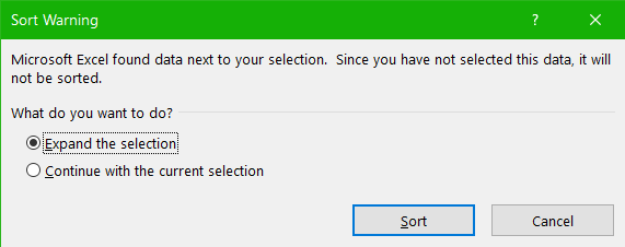
MedAttrib: author-generated. MS Excel Sort warning.

• What to do? Let’s choose “Continue with the current selection” then click the Sort button to observe what happens.

Review the two Opt-In columns. The J column one is out of order compared to the original I column. That is a problem.

Why did we go through this? Well, back in the Bronze Age when the author first worked with Excel, there were no warnings about sorts of data records in relation to a dataset that wasn’t actually connected as a table. The author hangs her head in shame at the data sorting mistakes that occurred. Now, even with the Excel sort warning, it can still be easy for an inexperienced data analyst to accidentally sort only part of a dataset, which would corrupt a batch of data when some information becomes untethered from its proper record. This would affect the data accuracy, the results of pivot summary tables, and definitely skew charts based on the data.

Let’s be more careful and try again.

• First, delete column J – the incorrectly sorted column.
• Next, select data from Column C, Cells C6-C36. This will give us the last names of customers.
• With this selection, again go to the Data ribbon, and select the Sort icon.
• Again, we will get the Sort warning. In this case, leave the default selected response of “Expand the selection”, then click the Sort button.

Now, Excel will select – for us – the entire range of data from Cell A6 through I36.

• In addition, the Sort panel gives us a choice of what to sort. In the Column Sort By field, choose CustLName.
• In the Sort By field, leave the default of Cell Values – Excel will sort based on the content rather than some other method.
• In to Order field, keep the default of A to Z.
• Click the OK button to generate the sort.

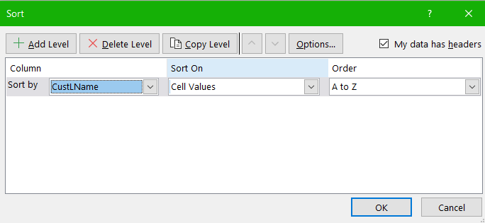
MedAttrib: author-generated. MS Excel Sort panel.

The whole data range of Cells A6-I36 should have been properly sorted, in A-Z order, based on the customer’s last name.

• SAVE your work.

Filtering data

Can we also filter data in a data range? Let’s find out.

• Place your cursor on any cell in the data range of Cells A6-I36.
• Choose the Data ribbon Sort & Filter group, and select the Advanced Filter button.

An Advanced Filter panel opens, which already displays the List range of A6-I36. That is efficient. So is the default option to filter the list in place. However, the filter requires some Criteria range to filter in or out. That requires us to give a specific data range – like one of the columns.

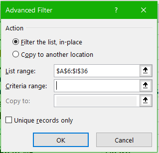
MedAttrib: author-generated. MS Excel Advanced Filter panel.

• Click inside the Criteria range field, then type f6:f36. This should select the State column in our dataset. Then click OK.

Hmmmm. Looks like nothing happened. Why? Well, in the end, we asked for a filter, yet the advanced filter didn’t really know what to filter for. Given that we were working with an unconnected dataset of rows and columns, Excel couldn’t comply. Let’s try something else.

• Place your cursor on any cell in the data range of Cells A6-I36.
• Choose the Data ribbon Sort & Filter group, and select the larger Filter icon. Something interesting happens. In the header row of our dataset, a bunch of small dropdown arrows appears. This tethers together the columns and rows, so that a filter can work with the range of A6-I36.
• Click the dropdown arrow in Cell F6.

You can see that the column can actually be SORTED. Yay! Let’s click the Sort A to Z.

• The whole dataset sorts to the A to Z of the States. Now, let’s filter out all states but Colorado (CO).
• Click the dropdown arrow in Cell F6. In the dropdown, Uncheck the Select all box. Then, put a checkmark only in the CO checkbox, and click OK.

There we have it; the dataset has had everything filtered out except Colorado. All the data still exists, but we can review only these two records until we clear the filter.

• To clear the filter, click the dropdown arrow in Cell F6. In the dropdown, choose the Clear Filter from “State”.
• SAVE your work, and close the file. EXCEL ACTIVITY #4 FINISHED.

Here is the really great news. Next, we will work with tables, so that we can utilize Excel’s connecting of data records in a range without having to go through some of these manual steps.

Tables

Even though Excel is all about data ranges, a very easy and useful way of accessing ranges of data is to simply convert them to an Excel table object. The table links record rows and columns together, and builds in formatting, sort and filter capabilities, a header and total row option, and can be named as a data range. Tables can be inserted from the Insert tab Tables group.

Turning a range of cells into an Excel table makes related data easier to analyze, visualize, and report. Structuring and planning table layouts are vital for data integrity. Below are guidelines to consider when designing and building a table from scratch:

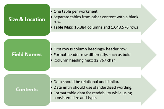
MedAttrib: author-generated. MS Excel Tables info.

ACTION: MS Excel Try Me Activity #5

Before you start, you should use your file manager utility to make a copy of the Excel_tablebasics.xlsx file that is in your DataFiles folder, then paste the copy into your Examples / MS_Excel folder.

Let’s open the file Excel_tablebasics.xlsx from the Datafiles MS_Excel folder. This is a variant on the previous Taste du Monde information with new names/records. The Page Layout theme should already be the Berlin theme and Aspect color palette, which will give us the colors to use in this activity. The workbook setup is for Narrow margins, horizontal orientation, and legal paper size.

Create a table

In the Excel_tablebasics.xlsx file, we have one worksheet: Customers. We want to take this dataset and convert it into an Excel table object.

Right now, we have a dataset with Row 7 that reads FirstName, LastName, Address, City, Region, PostalCode, and PhoneNumber.

• Select the data in Cells A7 through G30.
• With this range of data selected, go to the Insert ribbon, Tables group.
• In the Tables group, click the Table icon.

A Create Table dialog box should open, which should already have entered the data range of cells you selected into the ‘Where is the data for your table?’ field.

• Click the checkbox next to My table has headers, then click OK.
• The data range will now be encased in an Excel table. Now, let’s name the table, then change the table design.
• Click in the table, and then go to the Table Design ribbon. In it, overwrite the name Table1 with TMcustomers.
• With the Design ribbon still active, use the Table Styles group to choose Tan Table Style Medium 14.
• Adjust the width of the table columns so that the content doesn’t overflow.
• SAVE your work.

Context menu

• Click anywhere in the new table.

When you activate a table, a contextual Table Design ribbon opens near the top right of your Excel UI. Click on that tab.

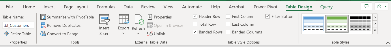
MedAttrib: author-generated. MS Excel Table Design ribbon.

The ribbon has several groups:

• Properties: Allows for naming and table resizing.
• Tools: Contains some table analysis tools.
• External Table Data: For use with linked live data sources, like a database that may have changes happen to it.
• Table Style Options: Basic table parts designation items.
• Table Styles: Color and layout styles for tables based on the Excel theme, color palette, and font palette you choose.

For our purposes, we will use the groups of Properties, Table Style Options, and Table Styles.

Entering & deleting records

Tables require constant updating and may need calculations. When your table needs updating you can add/delete data, by adding/deleting rows, or columns. Excel adjusts the table automatically to the new content. The format applied to the banded rows updates to accommodate the new data set size.

When calculations are needed you can create a calculated column or use the built-in Total Row tool. Excel tables are a fantastic tool for entering formulas efficiently in a calculated column. Excel allows you to enter a single formula in one cell, and then that formula will automatically expand to the rest of the column by itself. There’s no need to use the Fill or Copy commands. This feature can be incredibly time-saving, especially if you have a lot of rows. And the same thing happens when you change a formula; the change will also expand to the rest of the calculated column.

For now, we’ll just add a little data.

• Click into Cell A31, and type your own first name, then click your keyboard’s Tab button.
• In the next cell, type your own last name, then click Tab again.
• In the third cell, type a made-up street address then hit Enter. The table expanded its format and range down to accommodate the new row of text you entered.

TIP: Adding Rows. It can be tempting to insert blank rows further up in a table and add data, yet with the ease of sorting and filtering, that isn’t really an efficient way of adding data.

First, let’s add a column. We’ll want to add some budget numbers. We’ll just do the simple thing and add a default number so that we can move quickly.

• Click in Cell H7, which is to the right of the 7th header column title.
• Type ProductSales then click your Enter key. Cool! Excel just added a whole column of formatted space to our table.
• In Cell H8, type 25, then press Enter.
• Copy the contents of Cell H8, and paste the data into Cells H9 through H30.

Why did we do this? We want to add a total row to the table using the Table Design tab options.

Delete Table Columns

You can easily add and delete columns and rows to a table. Let’s delete a column we don’t really need – the PostalCode column.

• Click in Cell F7. Then click on the Home Tab, and look for the Cells group. In this group, click the Delete dropdown arrow, and from the list, choose Delete Table Columns. The PostalCode column disappears.

Total row

A useful table tool for data analysis is the Total Row. You can quickly total data in an Excel table by enabling the Total Row option, and then use one of several built-in functions provided in a drop-down list, per column. The Total row, which is added to the end of the table after the last data record, can calculate summary statistics, including the average, sum, minimum, and maximum of select fields within the table.

The Total row is formatted with values displayed in bold, the double border line option is separating the data records from the Total row.

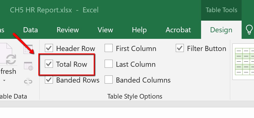
MedAttrib: Beginning to Intermediate Excel. MS Excel total row.

• Click anywhere in the Customers table, then choose the Table Design ribbon.
• In the Table Design, click the Total Row checkbox In the Table Style Options group. This will add a table row.

Excel redirects you to the bottom of the table to view the total row, where a SUM of 600 defaulted in the Prices column.

Let’s add a currency format using the Home tab Number group Number Format dropdown menu.

Another benefit of Excel table objects is that you can sort and filter columns without the data being mis-sorted, because the table locks a record’s data together.

Before we close this activity, let’s sort, then filter, the Customers table.

• Click anywhere in the Customers table.
• Sort the City column with the Filter button by opening the dropdown filter options and choosing Sort A to Z.
• Filter the State column with the Filter button by opening the dropdown filter options.
• In the options, uncheck the box for Select All.
• Then check the boxes for only CA. The table will have collapsed rows to show only the state CA, and the total for only those products.
• SAVE your work, and close the file. EXCEL ACTIVITY #5 FINISHED.

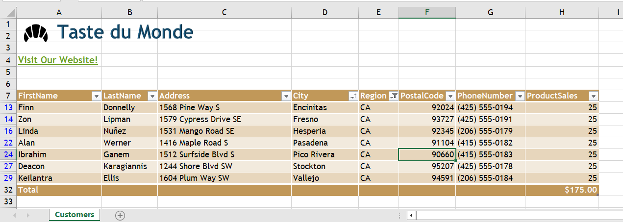
MedAttrib: author-generated Image of MS Excel table activity.

Calculations

This section reviews the fundamental skills for entering formulas into an Excel worksheet. The example used for this chapter is the construction of a personal budget. Most financial advisors recommend that all households construct and maintain a personal budget to achieve and maintain strong financial health. Organizing and maintaining a personal budget is a skill you can practice at any point in your life. Whether you are managing your expenses during college or maintaining the finances of a family of four, a personal budget can be a vital tool when making financial decisions. Excel can make managing your money a fun and rewarding exercise.

As a result, Excel is used for many kinds of calculations: mathematical, statistical, financial, scientific, reference lookups, and more. It is useful in many types of business, and is a key tool in cleaning, calculating, and analyzing data.

Formula Basics

A main strength of Excel is that you can use it to calculate data in many ways. Calculations allow for the development of additional data for analysis and decision making. A spreadsheet full of employees, their salaries, and the value of their benefits packages is useful. Calculating the annual and quarterly costs can be more useful in using for comparisons, preparing for taxes, etc.

Excel formulas are an expression that operates on values in a range of cells and return a result. They let you do calculations like addition, subtraction, multiplication, and division.

Excel functions are also formulas, but they are predefined and perform calculations by using specific values, called arguments, in a particular order, or structure.

Formula bar

We’ve used the formula bar a bit when not directly inputting data into Excel cells. The formula bar shows what is in a cell. However, its power comes from the ability to write and process formulas, to display named ranges and how the formula is organized, and in helping identify errors.

In the example, the formula bar is displaying a simple calculation for Cell A1. To the left of the field, the small fx icon is a way to open the Functions panel and access to the Excel functions library. The green checkmark is a way to approve a formula instead of simply pressing Enter. The red X is important because it allows you to back out of the formula bar without saving what is in it. Why is that useful? It can be all too easy to accidentally click in the wrong cell and corrupt a working formula, and the red X lets you stop before you can save and exact the corruption, error, etc.

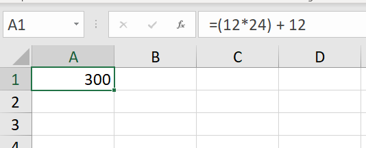
MedAttrib: author-generated. MS Excel formula bar.

Formula Ribbon

In Excel, you can manually input formulas, as we did in the chapter on linking to data cells. You can also use the Excel Formula ribbon to access common predefined functions and to look up a wide variety of functions in the Excel function library. This is also where we have found the Name Manager tools for naming ranges in a dataset. Those named ranges show up in formulas in a way that keeps a formula from seeming to access random and long strings of cell range information. The named ranges add context in a formula, especially for troubleshooting.

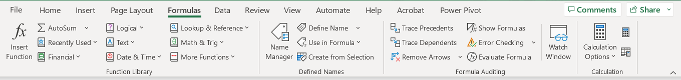
MedAttrib: author-generated. MS Excel Formula ribbon.

The Excel Function Library

Users can access the Function Library from the Formulas tab by clicking on the Insert Function icon. The Insert Function panel opens and allows for a search of formula-related keywords. You can also try to browse through the category dropdown. This is useful to people who work in specific industries in which they use a lot of calculations, whereas for basic workplace talent, most of the available functions won’t mean anything or be useful. The use is in context of one’s training in specific career areas requiring calculations.

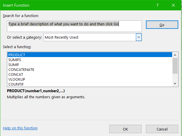
MedAttrib: author-generated. MS Excel Insert function / Function Library access.

Thinking out formula scenarios

A key part of succeeding in using any formula or function is to know exactly what you want to accomplish. Students in numbers and data-heavy fields are usually learning the skills for what calculation processes are needed, and Excel is a tool to accomplish that. Students in fields that don’t work with a lot of data or computations can find formulating the scenario, or words, for what needs to be calculated and why/how.

Steps

First, keep in mind that any calculation is a kind of combination of a story problem (UGH!) and a test of logic.

• How much is a “service”?
• What is a bonus for a high achieving real estate agent?
• How many products were sold in the last 3 months?
• How many days are in a class quarter?
• If you know someone’s name and look it up in a table, can you tell what region they represent or how much property they sold?

SO, the first thing you have to do is make sure you understand exactly what is being asked. Then you need to figure out what exactly you are trying to reference – to look at – so you can pull out the information you need. Then you need to ask Excel the right kind of question in terms Excel can calculate from.

Here’s something I learned when I first took a class in basic programming:

• Write out what I think I am being asked to do.
• Drink coffee (or fave beverage).
• Write out what steps I think I would need to do to get at the information.
• More coffee.
• Look up / research Excel information to see what types of calculations I need to do might require.
• Think about stronger coffee, but likely go for calming tea or water.
• Study the basic logic and format of a calculation to see if it can do what I need.
• Take a break for a serious treat or rest.
• Experiment.

Say you are being asked to get a total of the sales from the 8 sales reps who sell coffee to 3 cafes. You would figure (rightly) that you need to see a list of all their sales, then get a total of those numbers. You would be looking to get a grand totals response in terms of currency.

Say you need to find out which coffee roasts sold well over Fall 2022? you would need to figure out how to ask Excel to look up the column of roast flavors, see the quantities sold, and for the months of September, October, November, and December 2022. You would need more information to find out if you are supposed to find the count for each coffee, or the dollar amount sold, etc. Then you would need a way to either do a subtotal table, or a lookup table, etc.

Say you (as a teacher) have 30 students who have finished the class and need you to calculate their final grades. You need to know the students’ names, their final points, and some table of what points are equal to what publishable numeric grade. You would need to do some kind of lookup and have the response calculate into your student roster next to their point count so you could accurately update the school grades with the right numeric grade (4.0, 3.8, etc.)

You usually have to logically process what is being asked, and carefully decide what is needed. Take your time, map it out if you need to, and even write a layman’s English Language process. Then figure out how to ask Excel to calculate it for you. The Excel Functions menu ribbon and Functions lookup provides wizard windows for every function, so if you know what I need to look for, you can use those quite handily.

Parts of a formula

When you make a formula in Excel, there are several different components that supply the source data to the formula and express what operations should be performed on that information. Depending on the formula type, you may need include any or all of the following items:

• Starting the formula:  In order for Excel to know the cell content will be a formula to be calculated, you need to start by typing the EQUALS sign  = This tells Excel that the contents of the cell will be an answer to a question, rather than a string of text or a basic number to format in some way.
• Constants: Numbers or text values that you enter directly in a formula, like =2*3. This is a manual way of telling a formula what to calculate with.
• Cell reference:  A reference to a cell that contains the value (item) you want to use in your Excel formula, e.g. =SUM(A1, B2, C3). This allows you to create formulas that can be copied and reused, rather than requiring a manual input of the numbers yourself.
• Range reference: To refer to data in two or more contiguous (next to each other) cells, you use a range reference like A1:A5. For example, to sum values in all cells between A1 and A8, inclusive, use this formula: =SUM(A1:A8).
• Names: A defined name for a cell range, constant, table, or function, for example =SUM(TaxCol). In earlier chapters we created and used named data ranges in part to prepare for working with formulas.

Operators

Operators: These are special symbols that specify the type of operation or calculation to be performed, such as +, *, etc. They tell Excel what the operation, or calculation method, is to be, like sum, division, etc. For this chapter, we’ll only look at arithmetic.

• Addition: + (plus sign)
• Subtraction: – (minus sign)
• Multiplication: * (asterisk)
• Division : / (forward slash)
• Percent: % (percent sign)
• Exponentiation: ^ (caret)
• Equal to: =
• Greater than: > (greater than sign)
• Less than: < (less than sign)
• Greater than or equal to: >= (greater than or equal to sign)
• Less than or equal to: <= (less than or equal to sign)
• Not equal to: <> (not equal to sign)

The order in which calculation is performed can affect the return value of the formula, so it’s important to understand the order, and to use parentheses to change the order to obtain the results you expect to see. If a formula contains operators with the same precedence — for example, if a formula contains both a addition and subtraction operator — Excel evaluates the operators from left to right. Otherwise, you will want to use parentheses to separate/clarify sections of a formula. For instance, multiplication and division happen before addition and subtraction.

Excel uses the standard mathematical order of operations. When writing complex formulas it is important to remember this order of operations. You want to be sure that your formulas will calculate in the order you intend. To help you remember which operations will be performed first, you can use the acronym PEMDAS.

• P – parentheses
• E – exponents
• MD – multiplication and division
• AS – addition and subtraction

Cell References

Cell References are a way to refer to the contents of a cell.

• Absolute: Absolute references remain constant, no matter where they are copied.
• Relative: Relative references change when a formula is copied to another cell. This allows a formula to be reused and to pick up the contents of the record around it so that you don’t have to manually input all numbers (constants) yourself.
• Selection: You select one or more cells while creating a formula or a location reference in another table and/or worksheet.
• Named: You can Define a Name of a cell so that the cell remains stable in a formula that you copy and paste for further use in other cells in a column. This would be an Absolute reference. Otherwise, the pasted formula will change the cell’s location reference to be relative to the new row it is seeking to create the formula for. Example: =Fee*20, where the cell I5 has been named FEE, is more stable than =I5*20.
• Circular Reference: This happens when a formula is trying to calculate itself, and you have an Excel feature called iterative calculation turned off. It can also happen during indirect references in a formula. It results in errors.

Creating a Basic Formula

In this chapter, we will keep things straightforward and will work with basic mathematical formulas.

ACTION: MS Excel Try Me Activity #6

We will work with the Pets-R-Us sales workbook, named Excel_calculations.xlsx. Before you start, you should use your file manager utility to make a copy of the Excel_calculations.xlsx file that is in your DataFiles folder, then paste the copy into your Examples / MS_Excel folder.

Let’s open the file Excel_calculations.xlsx from the Datafiles MS_Excel folder.

In the Pets-R-Us sales file, we have one worksheet, which is more of a worksheet than a practical company ledger. Let’s start with the basic manual math.

The formulas begin with the = sign, to tell Excel something is being calculated, an answer will be provided.

• Cell B15 needs to add 12 and 12, which is a sum. In B12, type =12+12 with no spaces.
• Cell C15 can use this function instead: =SUM(12, 12)
• Cell B16 needs to subtract 978 from 2234, which is a difference. =2234-978
• Cell B17 needs to multiply 322 and 54, which is a product. =322*54
• Cell C17 can use this function instead: =PRODUCT(322, 54)
• Cell B18 needs to divide 330 by 10, which is a quotient. =330/10
• Cell C18 can use this function instead: =QUOTIENT(330, 10)
• SAVE your work.

Relative References

Relative: Relative references change when a formula is copied to another cell. This allows a formula to be reused and to pick up the contents of the record around it so that you don’t have to manually input all numbers (constants) yourself.

Now, let’s add some of the things in the Pets-R-Us table.

• Cell F6 needs to add Cells B6-E6, and because there are several numbers, the Excel formula that uses a Relative reference to those cells will do the job: =SUM(B6:E6)
• Cell F7 needs to add Cells B7-E7. Let’s copy the formula from Cell F6 and paste it into Cell F7 and learn what happens.

NOTE: Relative Reference. Copying the formula from Cell F6 and pasting it Into Cell F7, and having that change the formula to calculate the sum of Cells B7-E7, is an example of Relative References. Excel was able to adjust the formula to be relative to the data related to Cell F7, instead of simply copying the exact numbers from Cells B6-E6.

• Cell F8 needs to add Cells B8-E8. Copy the formula from Cell F6 and paste it into Cell F8.
• Cell F9 needs to add Cells B9-E9. Copy the formula from Cell F6 and paste it into Cell F9.

Now, we cannot do this for Cell F10. Why? Because Cell F10 is supposed to be the sum of Cells F6-F9, the cells above it in the column.

• Type =SUM(F6:F9)

Let’s get a little more experience and range. Rows 17-22 ask for a little more, and we’ll need to think about the order of operators – the order of what we calculate – when more than one calculation is happening in the formula.

• Cell B20: =F6-E6
• Cell B21: =F10*0.088
• Cell B22: =F10/2
• SAVE your work.

Before we calculate the next three, it would be useful to have a named data range instead of referring to the range of cells more manually. We did this kind of task earlier in this chapter, and in Excel_Calculations there is already one provided: RegionSums, for cells F6 through F9.

Now these three functions should work properly as typed:

• Cell B23: =AVERAGE(RegionSums)
• Cell B24: =MIN(RegionSums)
• Cell B25: =MAX(RegionSums)
• Then, lets also try B27: =SUM(B6:B9)*0.88
• B28: =SUM(C6:C9)/4
• SAVE your work.

Absolute References

Absolute references remain constant, no matter where they are copied. This is useful if you need one value (number) in a formula to remain the same no matter what rows of data are being calculated against it. We’ll do this with the Tax Needed cells in Column G.

However, in a formula, you have to explicitly tell Excel that the cell is a constant. An absolute reference is referred to differently in a formula / function. The idea is the tell Excel to freeze the reference so that it remains static – the same cell, no matter how it is used in a column that might otherwise auto-calculate relative references for you.

The Absolute reference format uses dollar symbol ($) before the cell’s coordinates to make them absolute. An example would be referring to the Cell G12 – a tax amount – as $G$12 in a calculation. Let’s try.

• Cell G6: =F6*$G$12
• Cell G7: Copy Cell G6 and paste in Cell G7. Notice the formula still refers to $G$12, which is absolute to Cell G12, which is what we want.
• Cell G8: Copy Cell G6 and paste in Cell G8.
• Cell G9: Copy Cell G6 and paste in Cell G9.

Again, we cannot do this for Cell G10. Why? Because Cell G10 is supposed to be the sum of Cells G6-G9, the cells above it in the column. Note: Even though we just used mixed formulas with relative and absolute cell references, the following formula does not need any absolute formula reference in it.

• Type =SUM(G6:G9)
• SAVE your work.

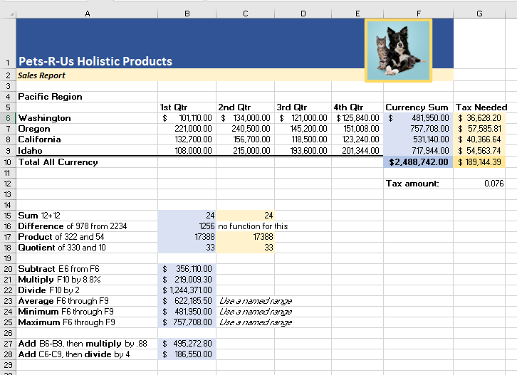
MedAttrib: author-generated. MS Excel Ch14 finished calculations.

Auditing Formulas

Excel provides a few tools that you can use to review the formulas entered into a worksheet. For example, instead of showing the outputs for the formulas used in a worksheet, you can have Excel show the formula as it was entered in the cell locations. This is demonstrated as follows:

• With the Excel_calculations.xlsx file open, click the Formulas tab of the ribbon.
• Click the Show Formulas button in the Formula Auditing group of commands. This displays the formulas in the worksheet instead of showing the mathematical outputs.

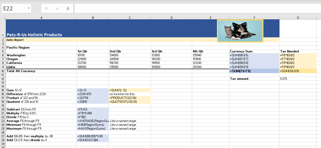
MedAttrib: author-generated. MS Excel Ch14 finished calculations showing formulas.

• Click the Show Formulas button again. The worksheet returns to showing the output of the formulas.
• SAVE your work, and close the file. EXCEL ACTIVITY #6 FINISHED.

You can also toggle Show Formulas on and off using the keyboard. Hold down the CTRL key while pressing the ` key. (The ` is known as the Tilde key and is to the left of the 1 key on your keyboard.)

Keyboard Shortcut: Show Formulas. Hold down the CTRL key while pressing the accent symbol .

Common Error Codes

Excel presents a number of error codes when a formula doesn’t work properly. And, for learners who work with Excel for standard/casual practice, the codes may not mean a lot or tell you exactly how to fix the problem. Excel tends to be somewhat obtuse in explaining a problem, because the explanation is general to the “type” of issue the program can’t resolve, not the exact nature of your actual formula and formula data.

These codes should give you something to start with,

• #DIV/0! Trying to divide by 0
• #N/A! A formula or a function inside a formula cannot find the referenced data
• #NAME? Text in the formula is not recognized
• #NULL! A space was used in formulas that reference multiple ranges; a comma separates range references
• #NUM! A formula has invalid numeric data for the type of operation
• #REF! A reference is invalid
• #VALUE! The wrong type of operand or function argument is used

Charts and Graphs

Pivot Tables

Pivot Tables are a data summarization tool. They are a bit complex and need a fair amount of practice time, so we won’t cover them in this chapter, although an instructor might choose to cover them with a video and exercises separately.

A pivot table can automatically sort, count total or give the average of the data stored in one table or spreadsheet and display the summarized data results in a second “pivot table”. Then the pivot table can have certain criteria in it filtered and organized so that the same data reveals different aspects of how it can be summarized. They tend to be listed with charts because part of a pivot table’s output often includes a companion chart.

Charts/Graphs – Insert tab

Charts allow for a visual representation of specific table data. They are not a static inserted item, like an image or shape. They represent live data that is being interpreted for analysis, like percentages of people who eat different desserts being shown in a pie chart. To create a chart in Excel you need to HAVE a table/table data to work with.

Charts can be initiated from:

• Pre-designed chart styles.
• Recommended charts based on the data Excel interprets.
• A chart created from specific data.

Charts, when clicked to be activated and using the Chart Design context tab or the Chart Format design tab, also allow for:

• Modifying chart info source location
• Chart formatting

Chart types

There are many chart types. Commonly-used ones include:

• Bar or Column charts: Show numbers that are independent of each other. Example data might include things like the number of people who preferred each of cold desserts, hot desserts, and no desserts.
• Line or Area graphs: Show how numbers have changed over time to demonstrate trends, like average summer times temperature in each region of the world.
• Pie or Doughnut charts: Show how a whole is divided into different parts, like the percentage of people who like cookies, cakes, baklava, cannoli, and fruit tarts. Y
• Scatter (XY) charts: They use plotted data point clusters to show correlations or patterns in data.

ACTION: MS Excel Try Me Activity #7

We will work with the Ihoosha Online Training supplies workbook, named Excel_charts.xlsx. Before you start, you should use your file manager utility to make a copy of the Excel_charts.xlsx file that is in your DataFiles folder, then paste the copy into your Examples / MS_Excel folder.

Let’s open the file Excel_charts.xlsx from the Datafiles MS_Excel folder.

In the Ihoosha sales file, we have one worksheet, which has one table from which we can derive charts. Let’s start with a Column chart, which can compare values across categories in no particular order of importance. The categories for Ihoosha are the quantity and cost, and what will be tracked is the average cost per student.

• Select the data in the table EXCEPT for the total row. A total row translated into a chart or graph can confuse the data and outcome. The data we need includes Cells A9-F20.
• Go to the Inserts ribbon, and the Charts group. Choose the Recommended Charts icon to access the selection dropdown.
• The Recommended Charts offers several options; select the first, a Clustered Column chart.

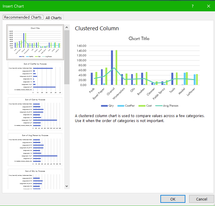
MedAttrib: author-generated. MS Excel Insert Charts panel, Recommended charts tab.

The chart will appear somewhere on your worksheet. Drag it just to the left of the table

When you click on the chart, the table range used in creating the chart is highlighted. Also, a contextual Chart Design ribbon and related Format ribbon (to its left) appear in the menu tabs.

• The Chart Design ribbon’s Chart Styles group lets you pick variants of the Clustered Chart format; Choose a variant format you like.
• You can change the base colors of the chart with the Chart Styles group as well. Click the color variation you like, keeping in mind that a chart should be easy to read and interpret.

You can also choose another chart type, but the point of a chart is to demonstrate specific data for a specific reason, so choosing charts for no particular reason isn’t solid Excel or data analysis process.

The chart-related Format ribbon allows you to make individual changes to elements of the chart, like the text boxes for the data, the lines, etc. At the left of the Ribbon a Chart Elements field can help you know what chart element you are on when you are making micro changes.

Let’s see if we can make a Pie Chart. Usually one of these summarizes one kind of data in percentages of the whole of the data, and this table may not really allow that. Let’s find out.

• Again, select the data in the table EXCEPT for the total row. The data we need includes Cells A9-F20.
• Go to the Inserts ribbon, and the Charts group. Choose the Recommended Charts icon to access the selection dropdown, but once on the dropdown, choose the ALL Charts tab.
• Look for the Pie Chart option, and notice that it does not show a preview. This means that this data can’t be used in the simple summary chart we want. We need to make a pivot table.
• Exit the Insert Charts panel, but leave your data selected.

A pivot table is essentially a summarizing table. It can get complex and summaries several things in several ways, depending on the Pivot Panel criteria you choose, which is why it needs some practice time. However, Recommended Pivot Tables can also give a simple summary table, which is what we need. Let’s see if we can get a summary of the Items or the Classes, and the average cost per student.

• On the Insert ribbon, Tables group, select the Recommended Pivot Charts icon.
• In the selection dropdown, look at the types of recommended summary tables offered. Let’s choose the Sum of Average Cost by Purpose recommendation, and determine if that captures what we want the first time. The Purpose is the title of Column 2 of the original table – the assignments.
• SAVE your work.

Yes, it does! It created a new sheet, called Sheet1, and placed the pivot table on that sheet. The chart is unformatted, as well.

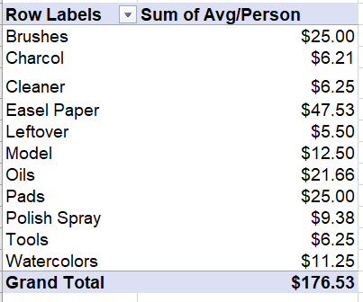
MedAttrib: author-generated. MS Excel summary pivot chart, unformatted.

• Go to Sheet1, and select the whole Pivot chart. Cut it, and copy it into the Action_Charts sheet a couple of lines below the main table.
• Delete the now empty Sheet1 worksheet.
• Click on the Pivot table. On the right side of the screen, a PivotTable Fields panel should appear. It shows that the two categories of data being summarized are the Purpose (the purpose of the materials being the assignments in Column 2), and the average cost per person.

We will not make changes on this panel, but you can look it over.

• Close the PivotTable Fields panel so that it is out of the way.

TIP: Pivot Table Fields Panel access. It can be reopened in the Pivot Tables Analyze ribbon, Show icon at the far Right. The Show Icon’s dropdown shows a Field List icon, which is what you choose to re-open the PivotTable Fields panel.

Let’s format the pivot table a little, manually. First, select all the numbers in the Sum of Avg/Person.

• If the pivot chart doesn’t already show currency, use the Home tab Number group to set these to currency.
• The pivot table columns look untidy in width for their content. Drag the right edge of Column A to the right so the Pivot Table’s first column is wide enough to see the data.
• Drag the right edge of Column B to the left so the Pivot Table’s second column is wide enough to see the data but not much more.
• Click in Cell A25, which reads Row Label. For simplicity, just overwrite the text with the phrase Supplies.

Now we have a Pivot summary table that might let us create a Pie Chart. Let’s find out.

• Select the data in the Pivot table, but not the total row.
• In the Insert ribbon, choose the Recommended Charts icon and look at the Insert Chart panel.

Look for the Pie Chart option on the lost on the left. It seems to have an available Pie Chart preview.

• Select the Pie Chart and click OK.
• The Pie chart appears on your workspace, and may need to be dragged so that it is positioned below the other chart.

The only issue is that the Pie Chart doesn’t label the percentages on the chart; the pie slices simply show them graphically.

• This is very simple to fix. Right-click on the Pie part of the Pie Chart, and select Add Data Labels.
• SAVE your work, and close the file. EXCEL ACTIVITY #7 FINISHED.

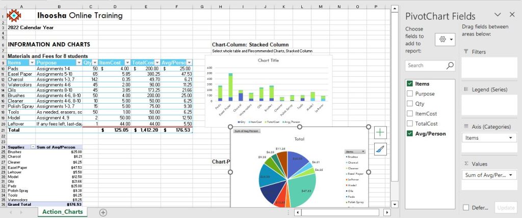
MedAttrib: Beginning to Intermediate Excel. MS Excel pivot chart and regular charts.

Review and Distribution

Review and distribution of your work is about preparing it for who will be consuming it. Will it stay in a Word document format, be saved as a PDF, printed onto paper, added as website content, populate an add or newspaper article, or be part of a book? It needs to be:

• Spell checked.
• Accessibility enabled (alt text, proper use of heading styles, accessibility for screen readers).
• Considerate of versioning.
• Have hyperlinks tested.
• Cited and attributed properly for intellectual honesty.
• Passed for plagiarism and other content integrity needs.
• Presented for readable print viewing.
• Secured for limited/no editing by others.
• If meant for team collaboration, prepared for making shared/trackable changes, comments, and notes.

Output/distribute work

• You can test and adjust your documents and review your content before it goes live by looking at the File/Print sections Print Preview and settings.
• In Excel, one worksheet can be printed separately from the whole workbook. Also, a whole workbook can be printed. Finally, you choose only some of a workbook’s sheets for output.
• You can make sure you have added metadata for web/online reference by updating information in the File/Info page.
• You can save files in different formats for distribution in the File backstage areas, like Save As (for current and older versions, RTF, text, and HTML), save as PDF, export, etc.

ACTION: MS Excel Try Me Activity #8

We will work with a Taste du Monde workbook, named Excel_ distribution.xlsx. Before you start, you should use your file manager utility to make a copy of the Excel_ distribution.xlsx file that is in your DataFiles folder, then paste the copy into your Examples / MS_Excel folder.

Let’s open the file Excel_distribution.xlsx from the Datafiles MS_Excel folder.

We have one worksheet, which has one table that needs to be set up for proper printing. This workbook my be emailed to someone, or shared on a SharePoint department site, or posted to a website, but any viewer might want to print it. The document has already had the margins, page orientation, and paper size established, and is designed to be printed wider-then-long on 8.5 x 14 inch sheets of paper.

NOTE: Things we covered in the MS Word chapter that behave much the same in Excel include the spell check, the accessibility check, and the Info Page review of metadata tags.

We need to look at two things in particular for Excel. The first is how the document will print out.

• Click anywhere in the document, then go to the File tab, Backstage area, and choose Print. The document has 2 printable pages, and as we review them, we can see that the columns all look about wide enough to see all the content.

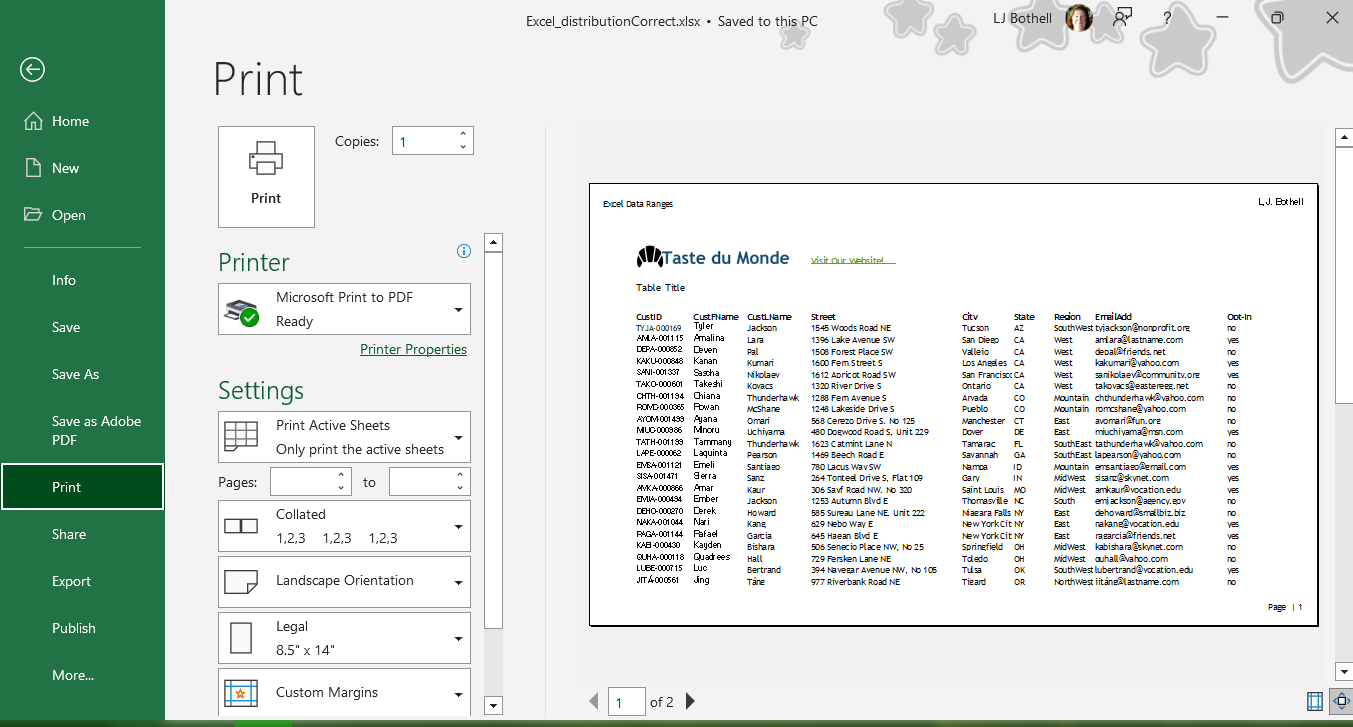
MedAttrib: Beginning to Intermediate Excel. MS Excel Print preview page.

• Exit the Print screen.

What if we don’t want to print all the columns? Let’s set a Print Area that does not include the last two columns.

• Select Cells A1 through G36.
• Go to the Page Layout ribbon, Page Setup group, and click the Print Area icon.
• In the Print Area dropdown, choose Set Print Area.
• Go to the File tab, Backstage area, and choose Print. The document still has 2 printable pages, and as we review them, we can see that the EmailAdd and the OptIn columns are not in the print preview.

Repeating column/row labels

One significant problem exists for what we see in the Print preview. The workbook has 2 pages, but only the first page shows the header row, which makes interpreting the second page difficult,

Now that you have fixed the cell and text formatting, you are ready to review the worksheet in Print Preview. You will notice that the worksheet is printing on multiple pages, and you cannot tell what each column of data represents on some of the pages.

• With Excel_ distribution.xlsx open, click anywhere on the worksheet.
• On the Page Layout ribbon’s Page Setup group, click the Print Titles button. The Page Setup panel will open to the Sheet tab.

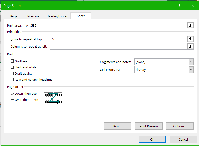
MedAttrib: author-generated. MS Excel Page Setup Sheet panel.

• Click in the Print Titles / Rows to repeat at top field. Be sure your insertion point is blinking in that box before moving on to the next step.
• In the worksheet, select Row 6, which is the header row of your table. The text $6:$6 should now appear in the Rows to repeat at top field.
• While still in this panel, also choose Page Order: Over, then down. While we hope that all out columns will stay on one “page”, if they do overflow it would be easier to sort if the tag-end page printed just after its main page, rather than at the end of the print session.
• Go to Print Preview (CTRL P) and look at each of the pages. Notice that the first header row is now repeated at the top of each page.
• SAVE your work, and close the file. EXCEL ACTIVITY #8 FINISHED.

This should give you a good overview of MS Excel skills that you can use in school and as a starter for basic workplace support tasks.