Chapter 10: Table Management
What We’ll Cover >>>
- Freeze Panes
- Basic Sorts
- Custom Sorts
- Custom List Sorts
- Basic Filters
- Criteria Filters
- Slicers
ACTION: Try Me activity
In this chapter, we’ll work with a mid-sized table from Taste du Monde again. Make sure you make a copy of the Ch10-TableMgmt.xlsx file from your DataFiles folder and save it into your Examples folder.
This is our goal for this work.
MedAttrib: author-generated. MS Excel Slicers.
Open the Ch10-TableMgmt.xlsx file from your Examples folder. It has one worksheet and a table with 17 columns and 174 rows. The table has already been formatted, named, calculated, and is ready for us to practice views and sorts.
Let’s look at various things we can do with tables.
Freeze Panes
We have worked a bit with simple sorts and filters, and we’ll practice more detailed versions. Before that, however, let’s find out a way to see some key data without quite so much scrolling. When one scrolls up and down in a big table (and loses sight of the header row), or across more columns than can fit on a single screen view, it can be easy to get lost.
Data sets can bridge thousands of records with dozens of fields and extend beyond a workbook window. It can be difficult to compare fields and records in widely separated columns and rows. One way of dealing with this problem is by dividing the workbook window into viewing panes by using the Split view option, then freezing certain rows or columns to keep them in place no matter where we scroll.
In our specific file the data set is manageable – barely – so freezing the first column, and the top header row could be useful when scrolling through data.
Using Freeze panes, or splitting windows, does not have any effect on calculations, a total row, or how a worksheet will print out. It is only a view aid.
- Click in Cell A5.
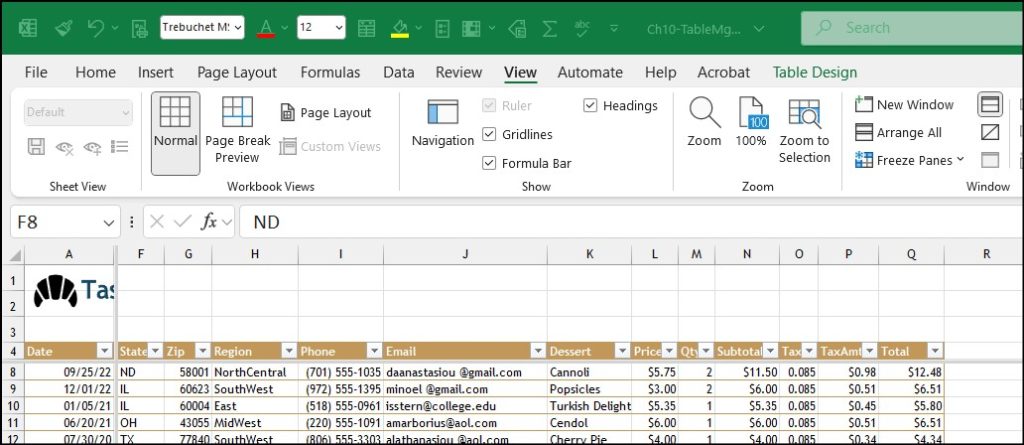
- Go to the View tab ribbon, and find the Window group.
- Click the Freeze Frames dropbox arrow, then select Freeze first column.
- Now, scroll to the right of the worksheet. Notice how the first column remains frozen in place while the rest of the sheet scrolls past.
- Click in Cell A5 again.
- Go to the View ribbon’s Window group, click the Freeze Frames dropbox arrow, then select Unfreeze panes. This clears the frozen panes view.
- Next, click the click the Freeze Frames dropbox arrow again, then select Freeze.
- Now, scroll down and see how the header row remains in place while the rows scroll up.
Now, what if we want to freeze both the header row and first column? This is a 2-frozen-pan operation, and takes a little more skill. We get to use the Split, then Freeze Panes options.
- Go to the View ribbon’s Window group, click the Freeze Frames dropbox arrow, then select Unfreeze panes. This clears the frozen panes view that froze the table’s header row.
- Click anywhere in the table, then in the View ribbon’s Window group, click the Split button. This will reveal a cross-section that seems to split the worksheet window into four panes.
- Use your cursor to grab and drag the horizontal line up until it rests just between the header row and the first data row (between Rows 4 and 5).
- Then, use your cursor to grab and drag the vertical line left until it rests just between the first and second columns (between Columns A and B).
- Next, click the click the Freeze Frames dropbox arrow, then select Freeze.
- Your document should allow for scrolling while leaving the first column frozen, and the header row also frozen.
This is efficient for very long and very wide tables.
MedAttrib: author-generated. MS Excel splitting frames before freezing them.
Basic Sorts
Sorting is one of the most common tools for data organization. By arranging data sequentially the information becomes more meaningful. Arranging records in a specific sequence is called sorting. If you sort by one column this is considered a single sort, which we worked on in Chapter 9. If you need to sort by more than one column, this is considered a custom sort. We already did a little sorting in earlier chapters, but sorting can be more complex than choosing one column and choosing A-Z.
The field or fields you select to sort are called sort keys. In Excel, you can easily – in one step – sort your table by ascending or descending order. Data in ascending order appears lowest to highest, earliest to most recent, or alphabetically from A to Z. Data in descending order in arranged by highest to lowest, most recent to earliest, or alphabetically from Z to A.
Excel will sort a range of data that is not in a table., which we reviewed in the chapter on data ranges. However, when working with large sets of information it is wise to make the data a table for integrity, and we have also covered. Excel locks the row of information creating a record, thus when sorted, the record remains intact, just reorganized. For example, when you sort the table by last name, all of the records in each row move together. It is always a good idea to save a copy of your worksheet before applying sorts. There are multiple places you can find and use sorting tools:
- When you first create a table, Excel automatically enables AutoFilter buttons; a tool used to sort, query, and filter the records in a table. The filter buttons appear to the right of the column headings. When you click the filter button sorting options appear on the menu options.
Sorts and filter options can be found in two ribbons. In the Home tab, in the Editing group, you can use the ‘Sort & Filter’ button, and then click one of the sorting options on the Sort & Filter menu.
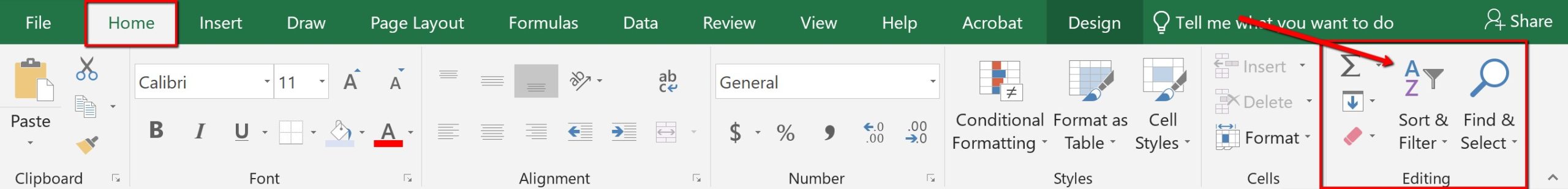
MedAttrib: Beginning to Intermediate Excel. MS Excel Sort and Filter Menu.
Also, from the Data tab, you can use the ‘Sort A to Z’ or ‘Sort Z to A’ buttons or for multiple levels select the Sort button to open the Custom Sort dialogue.
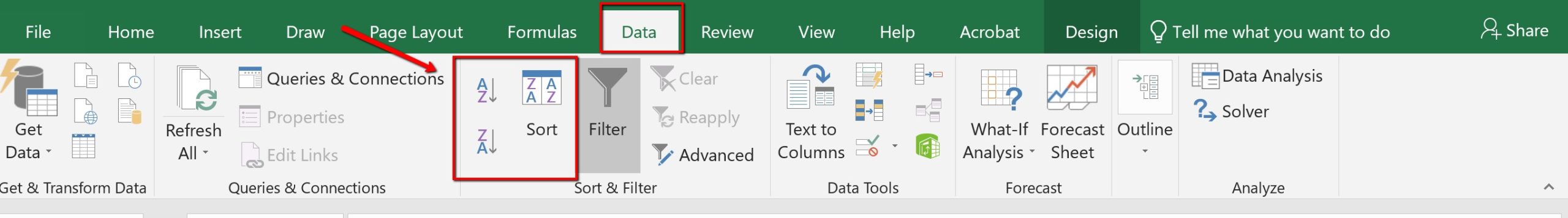
MedAttrib: Beginning to Intermediate Excel. MS Excel Data Tab Sort options.
Finally, you can right-click anywhere in a table, and then point to Sort on the shortcut menu to display the Sort sub-menu.
Let’s review with a single level sort.
- Click the Date column heading.
- Using the Home ribbon’s Editing group, click the Sort & Filter button, then A to Z.
Notice Excel arranges in chronological order all the Dates, keeping each record together. The filter button in the header row’s Date cell now displays an up arrow denoting an ascending sort.
Custom Sorts
Next, let’s try a 2-criteria sort. This allows us to sort a table by two important pieces of data (2 columns). The analyst looking at the Ch10-TableMgmt.xlsx file wants to consider data in the Region column, then in order of a dessert for that region.
When you need to sort by more than one level, you must use the Custom Sort option.
- Click anywhere in the table.
- Select the Data tab, and click the Sort button, which will open a Sort dialog box. Notice the last column sorted by is listed. We don’t want that, so we need to change the column heading name by dropping down the Sort by menu and selecting Region. Leave it at A to Z.
- NOTE: For the Mac, the custom sorting is available instead in the Excel/Preferences area. You specifically need to choose your Mac’s Excel button when in the Excel program, then choose Preferences, the Custom Sorts, and a window should open that allows you to add a new custom list.
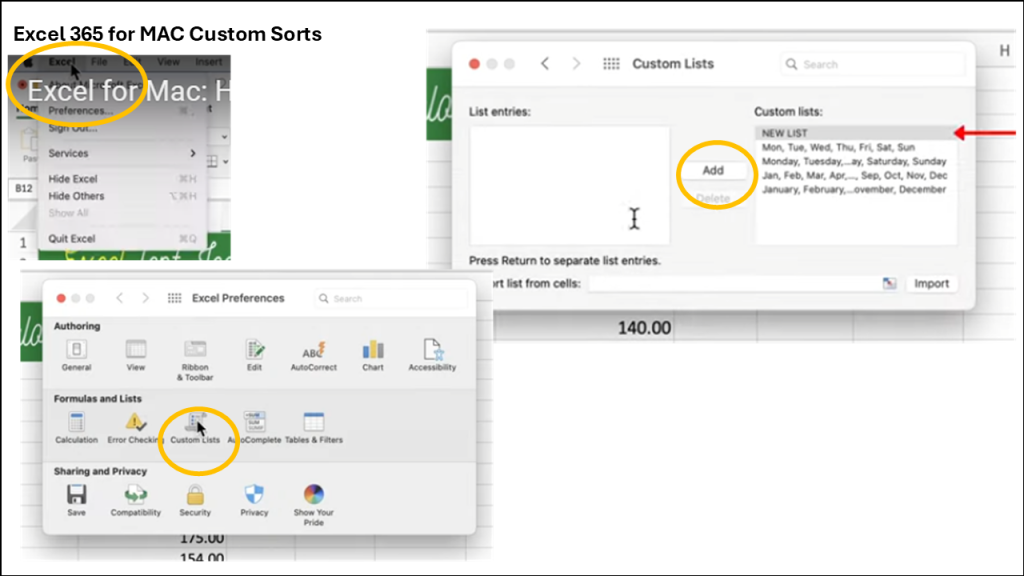
MedAttrib: Screenshots from Mike Thomas Excel for Mac YouTube video. MS Excel for MAC Custom Sort access.
- Then, while still in the sort dialog box, click Add Level.
- Mac Users: click the + symbol.
- Click the down arrow in the Then by section, and choose the column heading for Dessert. Leave it at A to Z.
- Click OK.
- SAVE your work as you go: Keybind is CTRL S / Mac CMD S.
Now the table is sorted by Region, and within the context of each Region, sorted also by the names of desserts from A-Z.
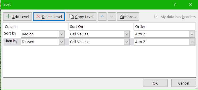
MedAttrib: author-generated. MS Excel Sort Dialogue Box 2-level.
This can be done for several sort levels, although in order to do that, an analyst needs a specific reason to sort data by more than a couple of criteria. Common combos in basic tables (not just this one) can be things like:
- Sort by region, then state
- Sort by state, then by city
- Sort by email, then opt-in
- Sort by salesrep’s last name, then region
- Sort by product, then category
- Sort by sales date, then product sold
Custom List sorts
When sorting you can create custom lists that allow sorting by characteristics that do not sort alphabetically. Example, text items such as high, medium, and low – or S, M, L, XL. Dates commonly require custom lists so you can vary in the way data is sorted by days of the week or months of the year.
In our case, we want to create a custom list that sorts regions, which is not in ascending or descending order. The analyst likes to order the regions based on the part of the country and wants to focus on the West US. And, the analyst wants to see the desserts related to these, and their prices.
Follow the below steps to create a custom list ordering:
- While clicked in the table, choose the Data tab and click the Sort button.
- In the Sort by row, click the drop-down menu in the Order Column for the Region heading. Choose Custom List.
MedAttrib: author-generated. MS Excel Custom List Dialogue Box 3-level.
- Click in the List entries: box and type West and press enter. Type Midwest, then enter. Type Southwest, then press Enter. Once all locations are entered, click Add. Then choose Ok.
- The second level sort can remain the same, because we want to still see the yummy desserts.
- Add a third level sort by clicking on the second level, then clicking Add Level.
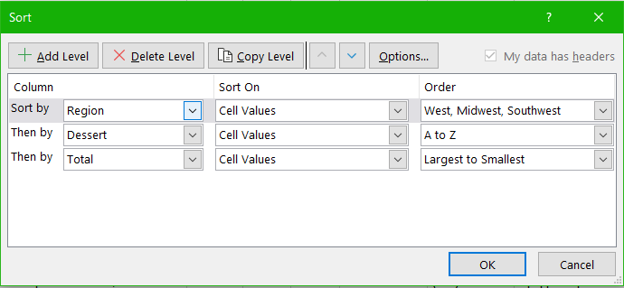
- For the third level, choose Total from the list so that we can see the costs of the desserts. The Order will default populate Smallest to Largest. Instead, change that to Largest to Smallest.
- Click OK to close the Sort dialogue box.
- SAVE your work as you go.
The custom sort is applied, and the table is now sorted by Region, using the custom order, then the dessert, and then by the Total column. The interesting thing is that we listed only three of the regions in our specific sort; the remaining regions simply sorted alphabetically after the sort list for Regions was applied. This allows us to see the three region areas as the priority of the whole table but also includes the remainder afterward.
Basic Filters
If your worksheet contains a lot of data, it can be difficult to find information quickly. Applying Filters is an effective way to temporarily and only show the information needed. Typically when filtering you are searching the data for specific information to filter the remainder out. Generally speaking, you are searching the data based on a question, or in other words, querying the data, and returning only the information that satisfies the question. The process of filtering records based on one or more filter criteria is called a query. Filtering data hides the rows whose values do not match the search criteria – but note – it does not delete the data of the hidden rows, and some actions you take may still try to affect those hidden rows, so be careful. The information that does not display is not deleted, it is just hidden, and will be redisplayed by removing the filter or applying a new filter.
An additional note is that when filtering rows that contain calculated numbers (such as in a total row), the calculated number will change to reflect only the calculations based on the visible rows.
Like sorting, Filter options are located in the filter button in each field name. By clicking the filter button, you can choose which values in that field to display, hiding the rows or records that do not match that value. The filter lets you choose to display only those records that meet specified criteria such as color, number, or text. In this situation, criteria is defined as; a logical rule by which data is tested and chosen. We applied a simple filter in Chapter 9 using the table header row filter buttons.
For example, you can filter the table to display a specific name or item by typing it in a Search box. The name you selected acts as the criterion for filtering the table, which results in Excel displaying only those records that match the criterion. The selected checkboxes indicate which items will appear in the table. By default, all of the items are selected. If you deselect an item from the filter menu, it is removed from the filter criterion. Excel will not display any record that contains the unchecked item. As with the previous sort techniques, you can include more than one column when you filter by clicking a second filter button and making choices. After you filter data, you can copy, find, edit, format, chart, or print the filtered data without rearranging or moving it.
Example: if you have a table full of cities in Washington State, and you want to only see Seattle and Spokane rows, you can filter out the rest by clicking only the filter button for those two cities.
Criteria Filters
The filters created are limited to selecting records for fields matching a specific value or set of values. For more general criteria, you can use criteria filters, which are expressions involving dates and times, numeric values, and text strings. Excel will identify what criteria filter to display based on the information in the column. For example, you can filter the employee data to show only those employees hired within a specific date range. Notice the criteria filter changes to Date Filters. If we were looking at the Current Salary column, the filter would be a Numbers Filter.
Using criteria filters, follow the steps below to search for customers who have spent a total greater than $7.00.
Identify customers by last name who spent more than $7.00 in the total column.
- While clicked in the table, clear any sort or filter applied by clicking the Data tab. In the Sort & Filter group choose the Clear button.
- Click the Filter button in the Total column. Select Number Filters, and choose the Greater Than criteria.
- Mac Users: uncheck the Select All checkbox before choosing the Between option.
- In the “Is greater than” field, type the number 7, then click OK.
- Sort the filtered table from A-Z by LName.
Notice the filter button displays a filter symbol and an up arrow indicating the column is filtered and sorted in ascending order. Also, notice that fewer rows are showing, and that the total row shows the total for only the displayed rows. Let’s narrow down the bigger spenders.
- Click the Filter button in the Total column, select Number Filters, and choose the Greater Than criteria. Type in 12. The result reveals fewer rows, and an adjusted Total in the total row for the spending of greater than $12.00.
- SAVE your work as you go.
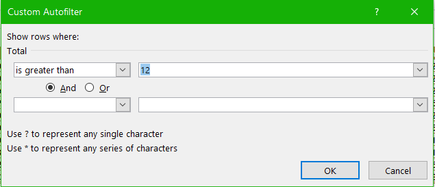
MedAttrib: author-generated. MS Excel Custom Autofilter.
Slicers
Another way to filter an Excel table is with slicers. Slicers, generally speaking, are visual filter buttons you can click to filter the table data. Slicers show the current filtered category, which makes it easy to understand what exactly is displayed. For example, a slicer for a field listing stores in several cities would have buttons for the Seattle, San Diego, Portland, and San Francisco locations.
When slicer buttons are selected, the data is filtered to show only those records that match the criteria. Multiple buttons can be selected at the same time, and a table can have multiple slicers, each linked to a different field (column contents). When multiple slicers are used at the same time, Excel uses the AND logical operator so filtered records must meet all of the criteria indicated in the slicer. When selecting multiple buttons in a Slicer, use the shift key to select adjacent field names. If the field names are not adjacent, use the non-adjacent selection method, pressing the CTL button, and selecting the field names needed.
The cool thing about slicers, though, is that they are a more easily visible way to change filters in a table instead of having to use the normal table header row filter buttons. By looking at the activated slicers, you can see at a glance what the filtering is, and at a touch, you can quickly change the criteria.
Note: See finished chapter activities image above to see slicers.
Follow the below steps to filter the table using visual Slicer buttons.
- Click in the Taste du Monde table area. From the Data tab, choose Clear to remove the current sort and filter applied to the data.
- Also, let’s clear the frozen view panes. Go to the View ribbon’s Window group, click the Freeze Frames dropbox arrow, then select Unfreeze panes. This clears the frozen panes view. Why? Because we will be adding rows, and row 4 will no longer be the header row.
- To make room for the Slicer buttons at the top of the table, we will add 7 rows between the title and the table area. Right-click cell A3. Choose Insert. Select Entire Row. Repeat these steps until the table header row starts in row A11.
- Mac Users: should hold down CTRL key and click cell A3. Then repeat until the table heading starts in row A11.
- Click back into the table area. Choose the Table Design tab, and in the Tools group, click Slicer. When the Insert Slicers dialogue box opens, click the Region and Dessert field names to display as slicers. Click OK.
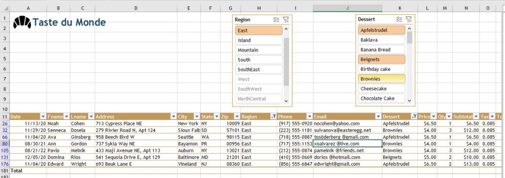
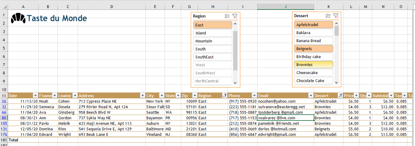
- Move, and re-size the two created Slicer boxes to fit in the approximate areas: Region around G/H 1-9, and Desserts around J/K 1-9. Make sure the buttons remain visible. Below is a visual example.
- From the Region slicer, click the West button. Notice the data filters to only show the data for the West region.
- From the Desserts slicer click Birthday cake. Notice the data filters to only show the data for Birthday cake in the West region. If there had been no matches, the table would appear empty except for the header row.
- Return to the Region slicer and clear it by clicking on the filter icon with the red x. Then choose both NorthEast and East. Note the non-adjacent selection method is needed. Select Northeast first, then press and hold the CTRL button on the keyboard, and then select East.
- Mac Users: hold down the CMD key not the CTRL key before you click on East.
- Change the Desserts slicer selection to Apfelstrudel, Beignets, and Brownies, using the same control/select as you did for the Region slicer.
The table results show there are 7 customers in the NorthEast and East regions who ordered those three desserts.
- SAVE your work, and close the file. We’re finished!