Chapter 11: Workbook Basics

What We’ll Cover >>>

• Adding/Deleting Worksheets
• Renaming Worksheets
• Copying Data to Another Worksheet
• Copying Worksheets
• Moving Sheets
• Grouping/Ungrouping Sheets
• Grouped Sheet Layout Settings
• Grouped Sheet Headers/Footers
• Worksheet Protection

We have already worked with a couple of Excel workbook files that included multiple worksheets. Depending on the version of Excel you are using, a new Excel workbook file may open with a default of one or several sheets.

TIP: Default sheets number. In the File Backstage Options area, under the General tab. You can also set the default number of sheets that new files will open with.

In this chapter, we will be working with a business file that contains information for an entire year. The file contains a worksheet for each quarter of the year, as well as a Summary sheet that will add info from all four quarterly sheets of data together. To begin with, we’ll get comfortable with moving through the sheets, organizing them, and making sure that all quarterly sheets are consistent.

ACTION: Try Me activity

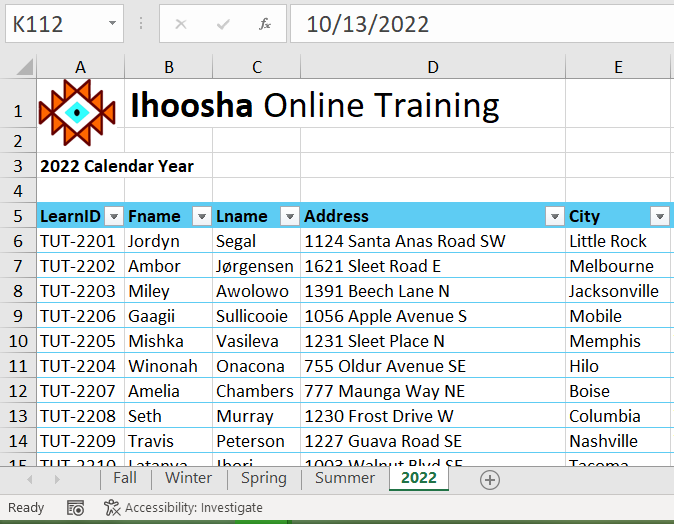
Ihoosha Online Training is a sole proprietorship business with a freelance online trainer. The data is about students from around the US, who enrolled for online asynchronous trainings in 2022. The data contains learner contact information, enrollment information, costs per credit, and a space (uncalculated) for grades.

Here is what we are aiming for (5 worksheets sheets total):

MedAttrib: author-generated. MS Excel workbook with multiple sheets.

Their Ch11–Workbooks.xlsx file currently has four worksheets. The 2022 table has already been formatted, named, and manually separated into three quarterly worksheets, and is ready for us to work on. We need another quarterly worksheet, and will learn a manual method of acquiring that information. One useful thing to know: Ihoosha is focused on a fiscal year of January-December of 2022, not an academic year of Fall 2021-Summer 2022. This will affect the order of things.

• Open the Ch11–Workbooks.xlsx file and save a copy to work on.
• Click on the different sheets at the bottom of the screen to move through the sheets. Notice also that all the quarterly sheets are identical in layout and format. Currently, 2022 is first, then Winter, Spring, and Summer.
• Fall – the last academic quarter that fell in 2022, has no sheet. It needs to be added.

Adding/Deleting Worksheets

Now, for practice, let’s add then delete new worksheets in this same file (workbook).

• Make sure you are in the 2022 worksheet, which has the full annual table. Click anywhere.
• In the worksheet’s name tab section, click the + button to add another worksheet tab, which should default name itself Sheet1. Sheet1 should appear just to the right of 2022.
• Click the + button to add a third worksheet tab, which should default name itself Sheet2 and appear to the right of Sheet 1.
• Click the + button to add a fourth worksheet tab, which should default name itself Sheet3 and appear to the right of Sheet 2.
• We actually do not need all of these sheets. Choose Sheet1, so that you are in that blank sheet, then look in Home menu ribbon for the Cell group.
• Click the down arrow on the Delete button and choose the Delete Sheet option from the drop-down list. This removes the Sheet1 worksheet.
  • Click the Delete button on the Delete warning box (if a warning box appears).
• Alternate method: RIGHT-click on the name tab of Sheet2, which will offer a contextual menu. On the menu, click Delete.
• This should still leave you with Sheet3.
• SAVE your work.

Keyboard Shortcut: Inserting New Worksheets. Press the SHIFT key + F11 key.

Renaming Worksheets

The default names for new worksheet tabs at the bottom of any workbook are Sheet1, Sheet2, and so on. However, you can change the worksheet tab names to identify the data you are using in a workbook. Additionally, using you can change the order in which the worksheet tabs appear in the workbook, and using that same process add a worksheet, delete one, protect one, etc.

The following steps explain how to rename and manage the worksheets in a workbook:

• Double-click the Sheet3 worksheet name tab at the bottom of the workbook. Type the name Fall.
• Press the ENTER key on your keyboard. Now we have a nice, empty sheet named Fall. We need to add some things into it.

Copying Data to Another Worksheet

First, this sheet should look like the others. Ihoosha already uses a specific Theme and color palette, and has a logo icon plus the company name at the top of worksheets. We need to copy that information from another sheet to this one.

• Enter the 2022 sheet, and in cell B1, copy the name Ihoosha Online Training. Then move to the Fall worksheet, cell B1, and paste the name into it.
• Re-enter the 2022 sheet, and copy the icon, then move to the Fall worksheet and paste it. You will likely need to drag it to the Fall sheet’s A1 cell space so it resembles the placement of other sheets.

Now, we need to acquire data from the 2022 sheet and copy/paste it into the Fall sheet. Let’s start with the header row of the table.

• In the 2022 sheet, select Cells A5-Q5, and copy them. Then move to the Fall sheet, place your cursor at cell A5, and paste. You should get a header row – without filter buttons – since this paste did not make this an Excel Table object.

We need to copy only the Fall records from the 2022 sheet to the Fall worksheet. Hpw can we make this easier to find so we can grab the correct into?

Pre-determining info to copy

Let’s do some conditional formatting in the 2022 worksheet to help visually determine what that data is before we actually copy/paste it elsewhere. Yes, we can and will sort the information, but assuming that Ihoosha chooses to use this sheet for 2023 later on, the conditional formatting can be even more efficient over the longer term, especially if the student base (number of rows of students) triples or more.

• Enter the 2022 sheet. Go to Cell K6, which is the first date in the Enrollment Date column. Let’s add conditional formatting, which will have to be created since it may not be a default Excel offering.
• On the Home tab Styles group, click the Conditional Formatting dropdown.
• Choose New Rule.
• Choose “Format only cells that contain”.
• In the Rule description, choose Format only cells with Cell Value.
• Make sure the second field reads Between, and in the third field type October, and type December in the fourth field.
• Click the Format button, which will open the Format Cells panel. In the panel, choose the Fill tab.
• In the fill tab, choose the light green from the 7^th column of the palette, second light green from the top. Click OK.
• Click OK in the Formatting Rule panel to accept it. Click OK on the Rule Manager if it is also still open, to apply the rule.
• SAVE your work.

Let’s find out what happens. Before we can get a result for the applicable dates, we need to apply this conditional formatting down the column.

Use the Home tab Clipboard group format painter to paint the format of cell K6 over cells K7 – K166.

Hmmm. . . that did not work. Why? It is likely because we looked at the value of the date cells, and Excel didn’t recognize that as a value that could be interpreted as October, December, etc. Well, mistakes are the stuff of learning!

• Select cells K5-K166.
• Open the Conditional Formatting dropdown and select Manage Rules to open the list of Conditional Formatting rules we have. There should be only the one we just created.
• Click Edit Rule, which will open up our rule instructions. Instead of October, replace that text with 10/01/22. Instead of December, replace that text with 12/31/22. Then click OK, then OK again to close the Rules Manager and apply the rule.

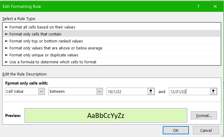
MedAttrib: author-generated. MS Excel Edit Formatting Rule panel.

Yay! That worked. And, since we applied the change in the rule formatting criteria to all cells in the table’s K column, the dates that met the rule complied and now have a light green background.

Now, let’s sort!

• Use the Enrollment Date table header’s filter button to Sort the column from Oldest to newest. Because the Fall quarter dates are the final months of the year, this sort puts them all at the bottom of the table, bunched together.

Now that we have the 2022 worksheet’s Fall months sorted together, we can easily see and choose to copy only the needed records and paste them into the Fall worksheet.

• Select only the records at the bottom of the table, with the green-background dates, which are for October-December 2022.
• Copy only the records from columns A-Q.
• Go to the Fall worksheet, and put your cursor at cell A6, then paste the information. This should paste in all the data you copied, starting at cell A6 and ending at Q66.
• Finally, we need this to be a real Excel table object, to make sorting/filtering smoother. Select cells A5-Q66, then use the Insert ribbon’s Table icon to insert a table with the header row checkbox checked.
• Click anywhere in the new table object, then use the Table Design tab Table Styles to select Turquoise Table Style Light 10. This will format the table like those on the other sheets.
• SAVE your work.

Copying Worksheets

Can’t we do this faster, with fewer steps? – says any student everywhere. Why yes, yes we can. Sometimes you will inherit a spreadsheet which requires more piecemeal tasks like we just finished, so that was of value to learn. However, we can also use a worksheet copy process instead of all these manual steps. Luckily, in this file, we already have done the work on the 2022 sheet with the conditional formatting for the date column, so that will help.

• First, click on the name tab of the existing Fall worksheet, and change the name to TEMP-Fall. We don’t want to lose our work until we are certain we don’t need it any longer.
• Then, enter the 2022 sheet. Right-click on the 2022 worksheet tab name.
• Select Move or Copy from the dropdown menu.
• In the Move or Copy panel, first put a checkmark in the Create a copy checkbox. This is so that the 2022 sheet will be copied, not simply moved.
• The To book field will show the name of the current file, since we are copying/moving inside the same file.
• Then, in the Before sheet, click (move to end) and click the OK button.

A copy of the 2022 worksheet is now at the right side of all the other worksheet name tabs.

• Double-click the 2022 (2) worksheet name, and type Fall to overwrite it.
• Click into this “new” Fall worksheet. It is already formatted, and all we need to do is to separate out the Fall months of October, November, and December – meaning, in this case, that we need to KEEP those records, and eliminate the remainder.
• Review the worksheet. Currently, all the October, November, and December records should still be grouped at the bottom, which means you need to delete the other records between them and the header row (which is row 5).
• Select Cells A6 through Q105, which are the record rows we need to delete.
• In the Home ribbon Cells group, use the Delete dropdown list and select Delete Table Rows.
• Now, the Fall sheet doesn’t need that conditional formatting. Select Cells K6 – K66, then in Home / Styles group / Conditional Formatting, choose Clear Rules, then Clear Rules from selected cells from the flyout sub menu. The conditional formatting for this sheet goes away.
• One more thing – let’s delete the TEMP-Fall worksheet that we don’t need anymore. Right-click on the TEMP-Fall worksheet tab name, and choose Delete. Accept the warning and delete it.
• SAVE your work.

Moving Worksheets

There are a couple of ways you can move a worksheet. We’ll try both, since the annual 2002 sheet should be at the end of the workbook, and the Fall worksheet should be at the beginning.

• Right-click on the Fall worksheet’s tab name. In the dropdown menu, select Move or Copy from the dropdown menu.
• In the Move or Copy panel, do NOT put a checkmark in the Create a copy checkbox. This is so that the Fall sheet will only be moved.
• The To book field will show the name of the current file, since we are moving inside the same file.
• Then, in the Before sheet, click 2022 (to move before that sheet) and click the OK button. The Fall worksheet should now be the first available worksheet tab at the left of all the worksheets.
• Press your mouse cursor down on the 2022 worksheet’s name tab, until you see a small icon of a sheet of paper floating near your cursor. That is the indicator that you can, while still pressing down on the mouse cursor, drag the worksheet tab.
• Drag the 2002 worksheet tab to the right of the Summer worksheet tab, then release the mouse/cursor. The annual 2022 worksheet should now be at the end of the row of worksheet name tabs.
• SAVE your work.

Grouping/Ungrouping Sheets

Most of your work will usually be one sheet at a time, but there will be times when you wish you could combine some work on multiple sheets at once. For a few things, like preparing for a print job, setting up all page layouts in a workbook, or selecting only some of the sheets for protection, you can. We will want to add headers and footers to our workbook on all the sheets, so temporarily grouping them for this work would be effective.

However, grouping worksheets in Excel is temporary. It can be ungrouped if you click on the name tab of one of the worksheets to navigate to the sheet to work on it. They will not ungroup if you work on the worksheet that is currently open in your workspace, but when you need to navigate away, they will ungroup. Let’s try this out.

• We are still working with the Ch11–Workbooks.xlsx file. Click once on the Winter worksheet’s name tab. Then, hold the control / command (Mac) key down, click on the Spring tab, then release the control/command key. Notice that both of those worksheet tabs change color, to indicate they are grouped.
• Click only on the 2002 name tab, and this will ungroup the other sheets.
• Now, click once on the Fall tab, then hold your shift key down and click once on the 2002 tab. This will group all five of the sheets.
• Click on any of the worksheet name tabs to ungroup them. Alternate method: right click on one of a group of name tabs, and choose Ungroup from the dropdown context menu.

Grouped Sheet Layout Settings

Let’s put grouping sheets to work for us by using this while creating header and footer content that should appear on every worksheet in the workbook. In this case, we want the Logo, company name, page number, and current date to show up on every page of the workbook.

Header: A header in Excel is the top-of-the-sheet area between the top of the margins for the sheet data, and the top edge of the sheet of paper/page itself. The space allowed is designated when setting up the page layout of a document.

Footer: A header in Excel is the bottom-of-the-sheet area between the bottom of the margins for the sheet data, and the bottom edge of the sheet of paper/page itself. The space allowed is also designated when setting up the page layout of a document.

TIP: You can work on Headers and Footers through the Page Layout ribbon’s Page Layout group’s Page Setup panel, OR you can work on them directly in the worksheet(s) by changing the sheet(s) view from the Normal view to the Page Layout view.

There are no side-of-page data fields like the header and footer.

Let’s group everything first, then check our margins, page size, and page orientation. This is covered in more detail in our chapter on Distribution. Enter the 2022 worksheet.

• Group all the worksheets by selecting the Fall tab, holding the shift key down, then clicking in the 2022 tab. All sheets should be grouped.
• You can work inside the 2002 sheet because it is the “open” sheet for editing in your workspace. Click once inside the sheet (not on the name tab).
• Go to the Page Layout tab, and in the Page Setup group, select the Margins icon. This will open the Margins dropdown.
• Click Custom margins, to see what the settings are.

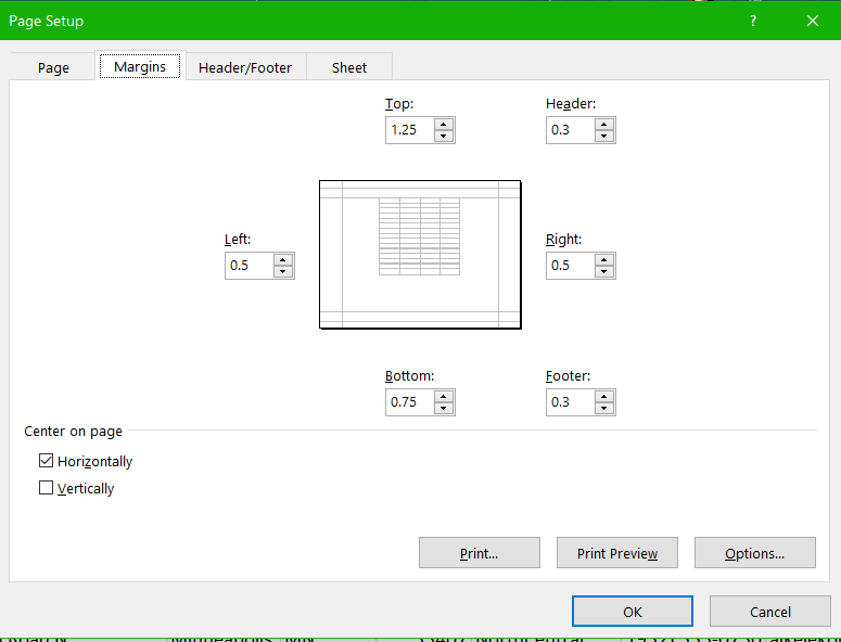
MedAttrib: author-generated. MS Excel Custom Margins.

We already have a top margin of 1.25 inches, a bottom margin of .75 inches, and side margins of .5 inches. The header and footer can be as close as .3 inches to the edge of the sheet of printed paper. Also, the content of any worksheet will be centered on the page when printed, even though in normal view we won’t be able to see that. We will keep these settings.

• Click Cancel to close the panel.
• With all the worksheets still grouped, click Orientation in the Page Setup group. It should show that Horizontal is selected. We will keep this.
• With all the worksheets still grouped, click Size in the Page Setup group. It should show that Legal (8.5 x 14) is selected. We will keep this.
• Now, with all the worksheets still grouped, look in the Page Layout ribbon tab, Sheet options group. Click the little button at the lower right of the group that will open the Sheet Page Setup panel.
• In the panel, click the Header/Footer tab.

Grouped Sheet Headers/Footers

Right now, the header and footer panel shows no header/footer content. Each has a dropdown arrow, which allows you to choose pre-set Excel content for either. Let’s personalize the header, and use a preset for the footer. This is covered in more detail in our chapter on Distribution

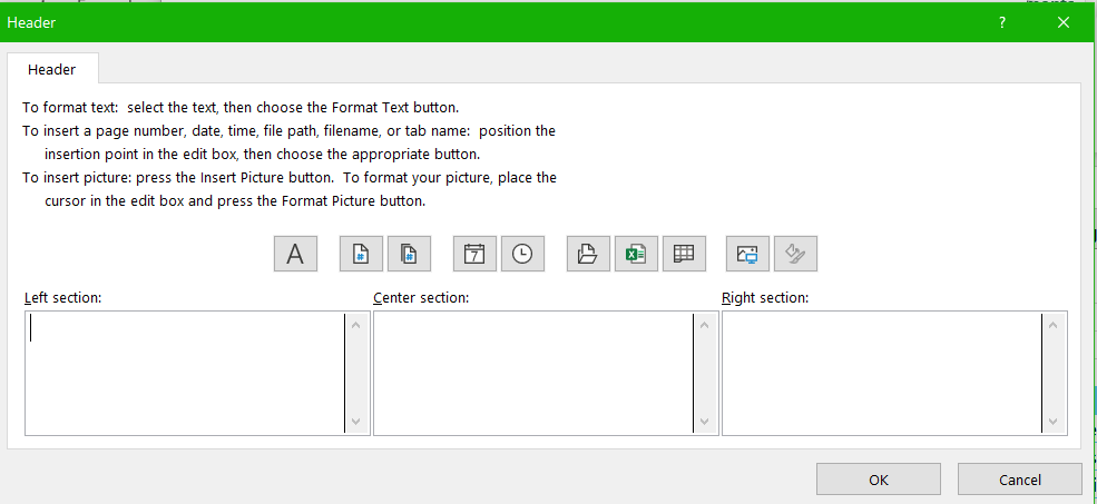
• In the panel, choose the Header button, which will open a custom Header panel.
• In the Header panel, click in the Left section, and type Ihoosha Online Training.
• While still in the Left section, select all three words, then click the Format Text button, which will open the Excel Font panel.
• In the panel, choose Font style Bold, and size 16, then click OK.
• Click OK again to exit the custom Header panel. Note how the Page Setup panel, which is still open, now shows your header information in the Header preview.
• In the Page Setup panel, click the dropdown arrow for the footer for a different way to approach the footer.
• Select the option Page 1 of ?, then click OK.
• In the Page Setup panel, the footer preview will show Page 1 of 1.

TIP: Excel update fields. In Excel header and footer content, some items may need to update to reflect the number of a page, or the current date. Excel adds code to do this in its date, page number, file name, and file path header/footer options. S, Page 1 of ? means that Excel will replace the ? with the proper page number when the worksheet is viewed in print or in Page Layout view.

• Click OK to exit the Page Setup panel.
• Ungroup your worksheets.
• Choose any worksheet, then choose the Page Layout view icon for it in the Excel status bar’s view option icons. In this view, with a little scrolling, you should be able to see the header and footer information on the sheet.
• On the same worksheet, return to Normal view.
• SAVE your work.

MedAttrib: author-generated. MS Excel custom header panel.

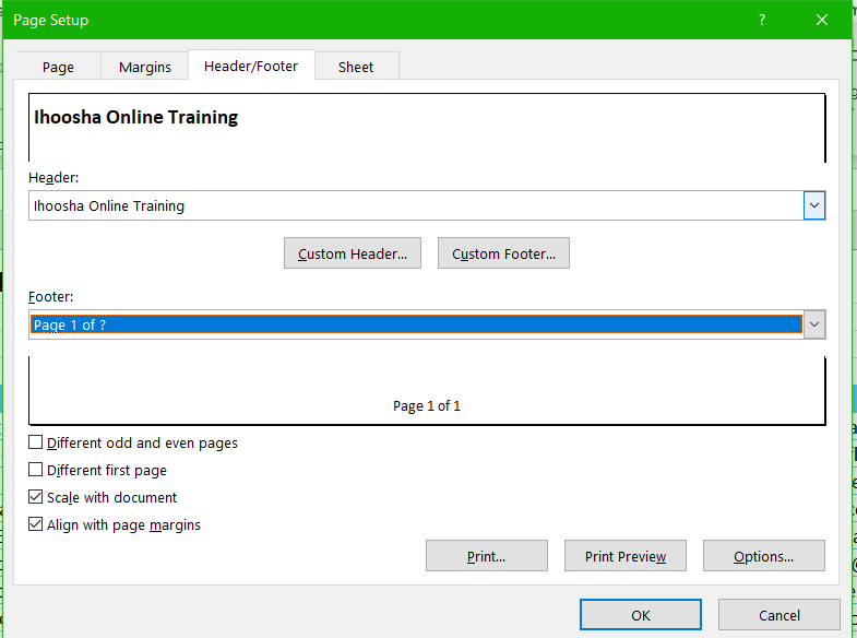
MedAttrib: author-generated. MS Excel Page Setup panel for headers/footers.

Workbook Protection

Let’s do one more task. This workbook is for all of 2022, and Ihoosha just finished Fall quarter, which means some work might be added to it. The other quarters are finished, and should be view-only, or protected from editing. Let’s do that.

• You would already have ungrouped the worksheets at the end of the last task. Now, shift click on the Winter, Spring, and Summer worksheets to group them.
• Right-click on your newly grouped worksheet tabs, which will offer a contextual menu. Interesting – the Protect Sheet option is grayed out.
• With the sheets still grouped, let’s go to the Review ribbon, Protect group, and. . . Hmmmm. The Protect Sheet is grayed out there too. The only available option is to protect the whole workbook.

In Excel for home and professional use, Excel only allows the protecting of one sheet at a time, or of a whole workbook. The Enterprise version has a multiple worksheet selection option, and there are macros that can do it, but for easy use, we’re stuck with one sheet at a time.

Learning from things we can’t do can be useful too.

• Ungroup the three worksheets. Then right-click on the Winter sheet, and choose Protect sheet.
• In the password field, type the word safe
• Don’t add any checkmarks in the list of choices,. Then click OK.
• When asked to repeat the password, type the word safe in again.
• Do the same steps to the Spring and Summer sheets.
• SAVE your work and close the file. We are done here!

TIP: Protecting work. Whenever you protect a worksheet in Excel, it usually means no one else can edit the worksheet (or workbook, if you protect the whole file). Be sure to know your protection password so you can unlock the sheet or workbook again.