Chapter 4: Data – Conditional Formatting

What We’ll Cover >>>

• Duplicate Values
• Text That Contains. . .
• Ranking Rules
• Range Conditions
• Color Scales
• Data Bars
• Icon Sets
• Corrections

Conditional Formatting in Excel allows you to visually identify patterns in data so that it is easier to analyze for patterns and trends. You can apply conditional formatting to a range of cells (either a selection or a named range), an Excel table, and in a Pivot table report (in Windows, not Mac).

NOTE: This chapter is presuming that learners are using the default Office color palette that Excel opens with. If you are using another one, you will need to go into the Page Layout ribbon, choose the Colors icon of the Theme group, and select Office.

The important thing with any conditional formatting is for it to be useful for observing and analyzing data. It should not get in the way of the data, or be used in ways that is a barrier to anyone with visual divergences who cannot see the formatting. Keep your conditional formatting very readable with good contrast colors and border line thicknesses, wider columns if needed, and use of conditions that don’t rely solely upon color differentiation to be useful.

ACTION: Try Me activity

This is what we will achieve in this chapter (image below). Please refer to it as you try the following activities. The instructions are for Windows PC and Mac users may have different UI locations for some of the commands. To work along, please download the starter file Ch4-Conditional.xlsx, open it, and save a copy of it to work on. This file is for Taste du Monde, an international specialty foods company, and we’ll look at a basic workbook for them. You’ll see them again later in the course!

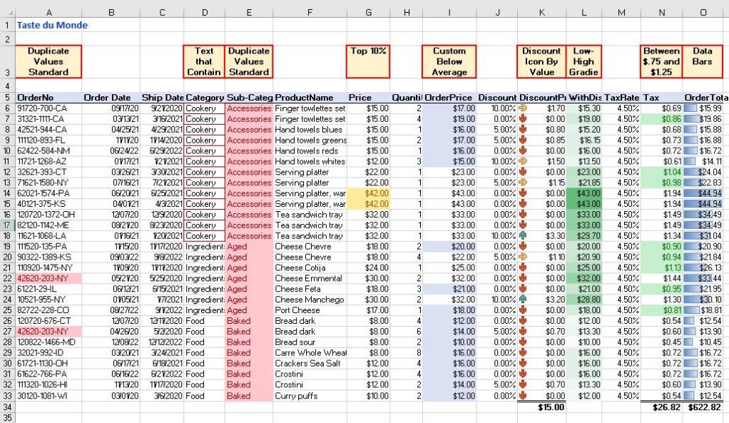
MedAttrib: author-generated. MS Excel Ch4-Conditional.xlsx final result.

Duplicate Values

First, let’s look at Duplicate values. Duplicate values are something you may need to see to determine if there is a pattern or an error in inputting data. Conditional formatting can help you “see” these things.

• Select Cells A6-A33 in the OrderNo column.
• On the Home Menu ribbon, look in the Styles group for the Conditional Formatting button.
• Press the button’s down arrow to see the choices available.
• Choose Highlight Cells Rules, then choose Duplicate Values.
• Click OK in the dialog box that appears. This will add formatting to cells that seem to be duplicates of other cells in the same column.
• Scroll down your Excel worksheet to see a couple of highlighted duplicates.
• This is a good use of Duplicate Values, because here you can see if the OrderNumber refers to the same order or possibly an input mistake. Hint: In THIS case, the duplicates are an error, since they refer to two different order dates.
• SAVE your work as you go: the Quick Access Toolbar shows a little disk icon, and the common keybind is CTRL S / Mac: CMD S.

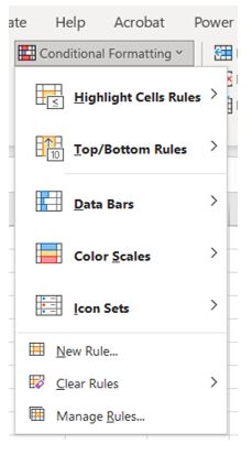
MedAttrib: author-generated. MS Excel Conditional formatting dropdown.

Try Another:

Select Cells E6-E33 in the Sub-Category column.

• Again choose the Conditional Formatting button
• Again Choose Highlight Cells Rules, then choose Duplicate Values.
• Again click the OK button.
• Now scroll down your worksheet, and see how ALL of the data cells in column E are highlighted.
• Note: This is not a good use of conditional formatting, especially if you are actually trying to ‘sort’ or ‘filter’ or otherwise work on specific data of like content/kinds. You would use Sorting or Filtering – to be discussed in a later chapter.

Text That Includes…

You may need to look for data that includes something specific, especially if you are working in a large worksheet and the data is buried in the content of a cell with additional information. This is a TEXT-Only task, not for numeric data.

• Select Cell D6 in the Category column.
• Choose the Conditional Formatting button, then choose Highlight Cell Rules.
• Choose Text that Contains…
• In the dialog box that opens, type the word Cook, then select the Red Border from the dropdown style options, then click OK
• Look at your worksheet. Cell D6 should have a red border around it.
• Next, let’s use this conditional formatting on the rest of the column.
• While in Cell D6, Click the Format Painter paintbrush in the Home Menu ribbon’s Clipboard group.
• Paint the rest of the column: cells D7-D33. This will apply the conditional formatting rule to all these cells, although only the ‘Cookery’ cells will be highlighted because only they will match the criteria.
• SAVE your work as you go: Keybind is CTRL S / Mac CMD S.

Ranking Rules

Top/Bottom formatting lets you get a feel of the importance of some percentage of numeric data. Perhaps you want to know the top 5% of the scores on a class test, or the 10% of students who seem to have the lowest scores and might need additional assistance. Here we’ll consider the prices for products at Taste du Monde.

• Select Cells G6-G33 in the Price column.
• Choose the Conditional Formatting button, then choose Top/Bottom Rules.
• Click Top 10%.
• In the Top 10% dialog box that opens, you can see that 10 is already selected in the Percent field – this number can easily be changed as one needs in future work. Keep this at 10.
• In the styles field, choose Custom Format.
• In the Format Cells panel, choose the Fill tab.
• In the Fill tab, choose a pale yellow background color. This should be in the 8^th column of the color palette, lightest yellow option. Click on it, then click OK.
• In the Top 10% dialog box, click OK.
• As you scroll down your worksheet, you should see two cells with the pale yellow highlight color.
• SAVE your work as you go: Keybind is CTRL S / Mac CMD S.

Average Conditions

Another option of Top/Bottom rules lets you see averages in some numeric data, such as to see if some products are underselling. Here we’ll consider the order prices at Taste du Monde.

• Select Cells I6-I33 (Column I – Cell I6 through Cell I33) in the OrderPrice column.
• Choose the Conditional Formatting button, then choose Top/Bottom Rules.
• Click Below Average
• In the Below Average dialog box that opens, you have only a formatting selection, including Custom. In the styles field, choose Custom Format. This will open a Format Cells panel.
• In the Format Cells panel, choose the Fill tab.
• In the Fill tab, choose a pale blue background color. This should be in the 5^th column of the color palette, lightest blue option. Click on it, then click OK.
• In the Below Average dialog box, click OK.
• As you scroll down your worksheet, you should see several cells with the pale blue highlight color.
• SAVE your work.

Range Conditions

Another option in Top/Bottom formatting lets you observe a specific and limited range of numeric information in a column. Here we’ll consider the prices for sales tax at Taste du Monde.

• Select Cells N6-N33 in the Tax column.
• Choose the Conditional Formatting button, then choose Highlight Cells Rules.
• Click Between.
• In the Between dialog box that opens, you can input values for the lower and upper range of what you want to consider – this number can easily be changed as one needs in future work. Type .75 in the first field and 1.25 in the second field.
• In the styles field, choose Light green fill with dark green text, then click OK.
• As you scroll down your worksheet, you should see several cells that qualify have changed color.
• SAVE your work.

Color Scales

Conditional Formatting Gradients lets you see a sort of ‘heat map’ of the range of all the numeric data in a cell. Here we’ll consider the with discount totals at Taste du Monde to see how they range in value.

• Select Cells L6-L33 in the WithDiscount column.
• Choose the Conditional Formatting button, then choose Color Scales.
• Click the Green-White color scale. This will instantly apply the conditional formatting.
• As you scroll down your worksheet, you should see a variation of greens to white in all the cells of the column. Note that we selected the 2-color green-white, instead of the full color range; this was simply because this particular activity worksheet is already stuffed full of eye candy.
• SAVE your work.

Data Bars

Instead of colorizing an entire cell, one might use small data bars to observe the difference in numeric data values. Here we’ll consider the with order totals at Taste du Monde to see how they range in value.

• Select Cells O6-O33 in the OrderTotal column.
• Choose the Conditional Formatting button, then choose Data Bars.
• Click the Blue Gradient Bars color scale. This will instantly apply the conditional formatting.
• As you scroll down your worksheet, you should see a bar of some length in each cell of Column O. This can look better and make more sense if your choose to make the column wider than just the content, especially if the bar seems to overlap any of the text. Remember, the important thing with any conditional formatting is for it to be useful, which means readable with good contrast.
• SAVE your work.

Icon Sets

One difficulty with Conditional Formatting is that much of it relies on color. There are, however, a lot of people who have some form of color perception divergence, and unless the conditional format color only uses high-contrast, and only 1 color selection to differentiate conditions, a color-divergent person may not be able to access and interpret the data. It can get in the way of actually seeing the data itself, too.

Excel doesn’t give many options, but the Icon sets can help. Many still depend on colors, but a couple give primarily ‘shape-oriented’ options, like the arrows used in our finished example above, and a couple more indicators’ choices. Even though these indicators use colors, the shapes themselves can be differentiated without color.

Here we’ll consider the Discount prices at Taste du Monde to see which are the higher discounts of 10%, medium of 5%, and no-discount price.

• Select Cells K6-K33 in the DiscountPrice column.
• Choose the Conditional Formatting button, then choose Icon Sets.
• In the Icon Sets samples, click the first of the Directionals – the 3 directions of arrows that are red, yellow, and green.
• As you scroll down your worksheet, you should see all the K Column’s data cells show an arrow that you could identify even if you cannot see color.
• SAVE your work.

Corrections

What if you have made a mistake with your Conditional Formatting? Or, do you want to delete it altogether? This is very easy to do. You can use the Conditional Formatting Manage Rules option.

• On the Home Tab, in the Styles Group, select Manage Rules at the very bottom of the Conditional Formatting drop-down list.
• Show formatting rules for: This Worksheet
• In the Conditional Rules Formatting Manager panel that opens, click once on the Duplicate Values for cells E6-E33.
• Click on Edit Rule, then click the format button.
• In the Format Cells panel, choose the Fill tab.
• In the Fill tab, choose a pale orange background color. This should be in the 6^th column of the color palette, lightest orange option. Click on it, then click OK.
• Click OK to exit the Format Cells panel, and click OK to exit the Conditional Rules Formatting Manager panel.
• SAVE your work and close your file. We’re finished!

TIP: Conditional Rules Formatting Manager. You can also choose to delete a formatting rule, duplicate one to change the data range and modify the style for it, and even to create a new rule that you could then apply to a data range you select.

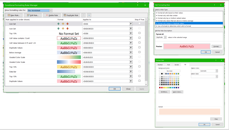
MedAttrib: author-generated. MS Excel Conditional formatting manager.