Chapter 15: Functions – Statistical

What We’ll Cover >>>

• Average Functions
• Count Functions
• Sum Functions
• Round Functions
• Value-finding Functions
• Time Functions

In this chapter, we will cover some statistical functions. Many of these are routine to general support functions in a number of businesses, and may also appear in some academic/training courses. Statistical functions are about calculating things like averages of data, counts of items, and sums of values. They are also basic mathematical functions that need additional criteria to clarify what is being calculated.

In review, formulas are various forms of calculations that can be developed and written as needed.

Functions are predefined formulas, of which Excel has many to make getting work done more efficient. Functions tend to fall into various areas of focus, like statistics, scientific, mathematic, financial, data retrieval, and more.

The components of a function are as follows: =FunctionName(Arguments)

• The Arguments are the criteria, such as the cells you are pulling data from, or the fixed values you type in (like numbers).

Functions are a type of formula, therefore they always start with an equal sign =

 

The next component is the name of the function. After the function name comes the arguments for the function, which are always enclosed in parentheses. The arguments are the cell locations and/or values that will be used in the function. The number and type of arguments varies based on the function being used, although in this section we will only work with a range of cells for the function arguments. Here are a few common ones for statistics:

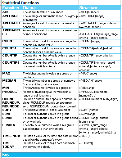
MedAttrib: author-generated. MS Excel Statistical Functions table.

In Excel, there are several methods for adding a function to a worksheet:

• Typing the function directly into a cell
• Using the Function Library on the ribbon
• Using the Insert Function button

ACTION: Try Me activity

We will work with a combination activities workbook, named Ch15-Stats.xlsx. Before you start working, go to your DataFiles folder and make a copy of the file for your Examples folder, then open that copy.

Our goal for this work is in two parts, and is shown further in the chapter.

The workbook has three sheets. The first is named Stats, and we can practice some of these functions unrelated to an example project. The second is named Ihoosha, and has a table of test scores for one of its online classes. The third is just a non-working  information sheet with a table of common statistical functions you can use for your reference.

Like previous formulas and functions we’ve worked on, these formulas begin with the = sign, to tell Excel that something is being changed and that an answer will be provided. Note that in some cases, the functions below may include the header row of the required table – but in others, the data part of the table, NOT the header row info, will be used.

Average Functions

Average functions are used to find the average, or arithmetic mean, of data. They are useful for looking at scores or other data that needs some kind of averaging.

Let’s consider Ch15-Stats.xlsx’s first worksheet, named Stats. We will use data from some or all of the tables on the sheet to calculate things requested in cells B15 through B31.

• Click on cell B15. To get the average of the list of numbers in the Amount table of numbers (cells A4-A13), use the AVERAGE function: =AVERAGE(A4:A13)

Note that, because the table of cells A4-A13 has been given the name tbl_Amount in the Table Design ribbon, the formula will interpret your A4:A13 instead as tbl_Amount[Amount]. This will happen in the rest of these tasks since in the Practice Worksheet all of the tables were given names in the Table Design ribbon. You can type in the cells I list, or you can select the range of data I list so that Excel picks up the range and adds it to the formula.

Click on cell B16. To get an average of only the numbers in the Amount table cells A4-A13 that are over 500, we need the AVERAGEIF function, which looks for one specific criteria (greater than 500) before it can calculate.

• Type =AVERAGEIF(A4:A13,”>500″)

Click on Cell B17. For this we will consider another table of mixed data – the Values table in column E. To get an average of only the numbers in cells E4-E13 fall between 55 and 1000, we need the AVERAGEIFS function, which looks in the whole one-column table for values of more than 55 and for values of under 1000 before it can calculate the answer.

• Type =AVERAGEIFS(E4:E13,E4:E13,”>55″,E4:E13,”<1000″)
• SAVE your work.

Count Functions

Count functions are used to do counts of data locations, like the number of items in a long spreadsheet meeting some specific condition. They are different than simply using filters, because they are about looking for data in the context of other data, not just sorting or filtering cell values. The data can be in numeric or text formats.

Click on Cell B18. To get a count of only the numbers in G column’s Counts table of mixed text and numeric data (cells G4-G13), use the COUNT function. It will count only the numbers, not the text.

• Type =COUNT(G4:G13)

Click on Cell B19. To get a count of the cats in the C column table of Items (Cells C4-C13) – which are strings of text, not numbers – we need the COUNTA function.

• Type =COUNTA(C4:C13)

Now we will work with a more complex multi-column table of movie information: the Sales table of columns I-N.

Click on Cell B20. To get a count of Sandy’s appearance in the movie Sales table – which is full of strings of text and numbers – we need the COUNTIF function. The COUNTIF needs to look for one specific criteria (Sandy’s name) before it can calculate.

• Type =COUNTIF(I4:I13,”Sandy”)

Click on Cell B21. To get a count of specific movies that sold for $9.99 in the Sales table, we need the COUNTIFS function. This looks for more than one specific criteria: the quantity of the films, and the price of the films) before it can calculate.

• Type =COUNTIFS(K4:K13,”>100″,L4:L13,”=9.99″)
• SAVE your work.

Sum Functions

Sum functions are used for adding data. Some of the data may need to meet specific conditions beyond just being a sum field at the end of a row or column of numbers, and a couple of more complex Sum-related functions can draw these out.

• Click on Cell B22. To get the SUM of the prices listed in the Sales table ( including the header), use the SUM function: =SUM(L4:L13)

Click on Cell B23. To get an SUM of only the quantities of films sold by Shanon in the  Sales table, we need the SUMIF function. This looks for one specific criteria (Shanon in the Salesperson column) before it can calculate her quantity of sales from the K column.

• Type =SUMIF(I4:I13 ,”Shanon”, K4:K13)

Click on Cell B24. To get an SUM of only the DVDs of Good quality, we need the SUMIFS function. This looks for more than one specific criteria before it can calculate. It will look at the quality of the film type DVD and return a sum of the related prices from the Price column.

• Type =SUMIFS(L4:L13,M4:M13 ,”DVD”,N4:N13,”Good”)
• SAVE your work.

Round Functions

Round functions are simply used to present data in some form of rounding of to a specific number of digits. In math, numbers aren’t just whole; calculations can take numbers to several or dozens of numbers past a decimal point, and rounding can bring this under more manageable control. This is how we get that the value of PI seems to represent 3.14, rather than 3.14159265359.

• Click on Cell B25. To round up the contents of cell L10 with no decimal points, type =ROUNDUP(L10,0)
• Click on Cell B26. To round down the contents of cell L10 with no decimal points, type =ROUNDDOWN(L11,0)
• SAVE your work.

Value-finding Functions

Value-finding functions in statistics are about determining the placement of data – high, or low, or median placement. This can be used in determining percentiles, like in assessing salaries, scores, demographics, etc. Our example is very simple, but these formulas are designed to be used with much longer ranges of data.

• Click on Cell B27. To look for the minimum number that appears in the one-column Amount table, type =MIN(A4:A13)
• Click on Cell B28. To look for the maximum number that appears in the one-column Amount table, type =MAX(A4:A13)
• Click on Cell B29. To look for the median (middle-value) number that appears in the one-column Amount table, type =MEDIAN(A4:A13)
• SAVE your work.

Time Functions

While Excel offers time functions in its Header and Footer options (like in the footer the date of a document being opened), you may find a need to note a specific time or date in the content of a worksheet.

• Click on Cell B30. To have Excel tell us what the exact time and date of right now is, type =NOW()
• Click on Cell B31. To have Excel tell us what today’s date is, type =TODAY()
• SAVE your work.

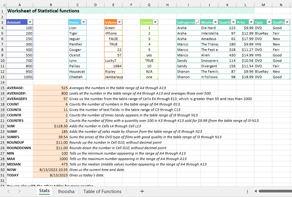
MedAttrib: author-generated. MS Excel Statistical Functions worksheet.

Practical Use

Let’s put some of this into practical use, so that we can see some outcomes of a valid table of data. Go to the 2^nd worksheet in Ch15-Stats.xlsx which is named Ihoosha. This contains a table of some student test scores, course points, and class costs. We can do some calculations in the table, and then use the worksheet-like area below to consider some Count and Values-based functions that are relevant to this kind of data.

First, let’s review the table to comprehend what is needed. There is the primary table of cells A4-H19 called Table1, with input data, which uses the Excel Turquoise table format. There is a portion of the table with a light gray background to separate the contents from most of the values that will be calculated with. There is the E column that has a light orange background, for calculation results of Student Averages. The F column has a light green background for more calculations, of Weighted Averages.

NOTE: While this table has been set up with the data formats already in place, in real life you will usually need to format numbers in various columns yourself.

Let’s get the average of student Latanya’s three test percentages.

• Click on cell E5.
• Type =AVERAGE(B5:D5) to calculate the average of her three scores.
• Copy the results of cell E5 down into cells E6-E17, so that the other student averages are also calculated.

Click on cell F5. Here, we need to do a complex sum of three items in one calculation. This is actually just a sum; however, we need a mixed-reference formula (some relative references for the scores, and absolute referencing for the specific test weights from row 19). These weights tell us that, regarding the importance of the tests in the student scores, test 1 and test 2 are each worth 25% of the accumulated total test points, and test 3 is worth 50% (it is likely a final exam).

• In cell F5, type =SUM($B$19*B5,$C$19*C5,$D$19*D5)

This has us add the products of Latanya’s 1^st test score to 1^st test weight, 2^nd test score to 2^nd test weight, and 3^rd test score to 3^rd test weight. Next, let’s finish off for the remaining students in the table.

• Copy the results of cell F5 down through cells F6–F17.
• SAVE your work

Now the table is complete. Let’s get to the additional worksheet fields in cells A22 through A31. This will allow us to gather more useful information about the students’ scores and performance from their table data and calculations. The cell ranges used in this section will refer to the actual data cells in the table, not the header row or the grayed-out test averages/weights rows.

• In cell B22, calculate the Count of students. This should use a COUNTA formula (for text) and reference cells A5 – A17.
• In cell B23, calculate a count of Test 1. This should use a COUNT formula (for numbers) and reference cells B5 – B17.
• In cell B24, calculate the number of students whose Student Average was greater than 80%. This should use a COUNTIF formula and reference cells E5 – E17.
• In cell B25, calculate a count of students whose Course Points fell below 250. This should use a COUNTIF formula and reference cells G5 – G17.
• In cell B26, calculate an average of student Course Points. This should use an AVERAGE formula and reference cells G5 – G17.
• In cell B27, calculate the minimum percent received for Test 3. This should use a MIN formula and reference cells D5 – D17.
• In cell B28, calculate the maximum percent received for Test 3. This should use a MAX formula and reference cells D5 – D17.
• In cell B29, calculate the middle percent received for Test 3. This should use a MEDIAN formula and reference cells D5 – D17.
• In cell B30, calculate the sum of the Student Costs. This should use a SUM formula and reference cells H5 – H17.
• In cell B31, calculate the sum of the Student Cost for only students who passed with 220 points. This should use a SUMIF formula and reference cells G5 – G17 and cells H5 – H17.
• SAVE your work and close the file. We’re finished!

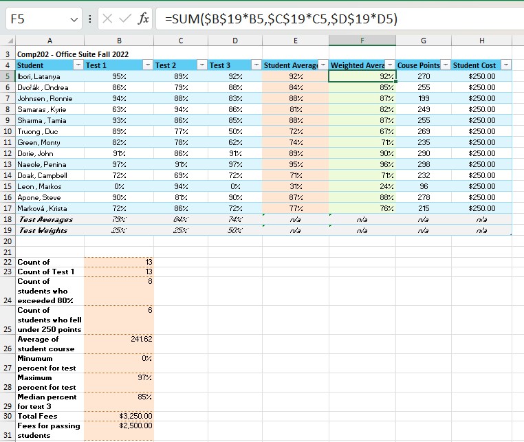
MedAttrib: author-generated. MS Excel Statistical Functions table of test scores.