Chapter 3: Data – Formatting for Analysis

What We’ll Cover >>>

• Text Formatting
• Cell Merges
• Dataset Formatting
• Text Effects
• Number Formatting
• (Auto)Sum Feature

This section addresses formatting commands that can be used to enhance the visual accuracy and appearance of worksheets. It also introduces a very basic mathematical calculation. These skills  will highlight how Excel can be used to prepare spreadsheets to help evaluate information and make decisions with the data.

ACTION: Try Me activity

TIP: Working with book files. In each chapter’s Try Me activities, you should make a copy of the requested data file that you extract from this textbook’s companion datafiles.zip folder. You should save it on your computer so you can save your changes, find it again, and reference it in the future if needed. Learners should use this tip while working through Try Me activities in each chapter.

For this chapter, we will use the data file Ch3-Format.xlsx in order to demonstrate the various steps. For data file download and saving information, please refer to the chapter Book Resources information.

Text Formatting

There are several fundamental formatting skills that will be applied to the workbook that we are developing for this chapter, like text and number formatting, adding visual touches, a basic calculation, etc. The basic worksheet formatting tasks can mostly be found on Excel’s Home menu Tab/ribbon. Note: this chapter focuses on the interface for the MS Windows operating system for PC, and Mac users will likely see similar icon/commands arranged a little differently.

The Windows for PC Excel’s Home ribbon currently has 9 groups of collected commands/icons. In this series of tasks, we’ll work with the Clipboard, Font, Alignment, and Styles groups.

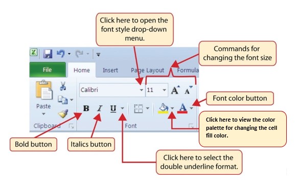
MedAttrib: Beginning to Intermediate Excel. MS Excel Font Group of Commands.

To get started, open the Ch3–Format.xlsx file. This is the look we will be working to accomplish:

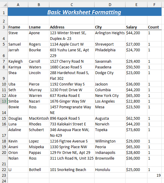
MedAttrib: author-generated. MS Excel Ch3-Format.xlsx final result.

You will find there is more than one way to do most tasks in Excel, and while the work-through here may list one method, please explore.

Text size and styles

First, we’ll work on Row 1, which is a document identifier title that lets a viewer know what the data they are seeing represents.

• Select cell A1. When active you will be able to see its contents showing in the formula bar.
• With cell A1 active, choose the Text size in the Home ribbon’s Font group and select 18. This makes the text a larger 18pt size.
• Then, from the same Font group, click the buttons for Bold, then Italic, then Underline.

Keyboard Shortcut: Text Formats. Hold down CTRL key while pressing the letter B (Bold), or I (Italic) or U (Underline) / Mac: hold down CMD key instead.

Cell and text colors

You can emphasize a region of a spreadsheet by adding color to the cells and/or text.

• Select the cells A1-F1. You may see the contents of only A1 in the formula bar, but you should also see a selection outline around the 6 cells you chose.
• Find the paintbucket Fill Color icon on the Home ribbon’s Font group, and click the down arrow on its right side. This will show you a color palette to choose a cell color from.
• If you hover over the colors, a tooltip will appear with the color’s information. Click on Blue, Accent 5 Darker 25%, which should be the second to the last column of colors, and second from the bottom of that column. OR, choose another dark color you like from the palette.
• Click only cell A1 again. Then using the Font Color button on the ribbon’s Font group, click the down arrow on its right side. This will show you a color palette to choose a text color from. Select White.

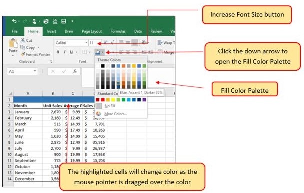
MedAttrib: Beginning to Intermediate Excel. MS Excel Fill Color Palette.

Merge Cells

Data is entered solely into one cell at a time, like in this activity file example’s rows and columns. However, for stylistic purposes, data can also be merged into more than one cell. For instance, the Merge & Center command is used to center the title of a worksheet directly above columns of data.

• Select cells A1-F1 again.
• Click the arrow on the Merge & Center button in the Font section of the Home ribbon to select the Merge & Center setting.

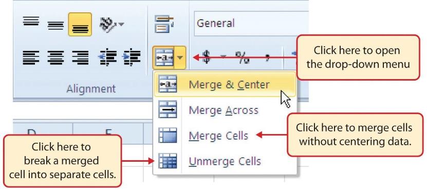
MedAttrib: Beginning to Intermediate Excel. MS Excel Merge Cell Drop-Down Menu.

• SAVE your work as you go: the Quick Access Toolbar shows a little disk icon, and the common keybind is CTRL S / Mac CMD S.

Dataset Formatting

Header rows

Any range of data in Excel that you may want to sort, filter, and/or calculate is considered to be a data set or data range. In order to help a viewer know what the data is for, a data range should include some kind of  Header Row. This is a row that you use to identify the expected contents of the columns of data (with the names of the columns, like FirstName, LastName, etc,). Sometimes you may see instead a header column, but for this course the norm will be the header row above columns.

The header row should stand out from the rest of the range of data for ease of identification. Let’s do that here.

• Select cells A3-F3.
• Using the Home tab’s Font group Bold icon, make these cells Bold.
• With the A3-F3 cells still active, click the Font group Border button’s arrow and select Bottom Border.
• SAVE your work as you go: the Quick Access Toolbar shows a little disk icon, and the common keybind is CTRL S / Mac: CMD S.

Borders

In Excel, adding custom lines to a worksheet is known as adding borders. Borders are different from the visually clarifying grid lines that appear by default on a worksheet to define the perimeter of the cell locations. The Borders command lets you add a variety of line styles to a worksheet that can make reading the worksheet data much easier. Here is a method for adding preset borders and custom borders to a worksheet:

• Click the down arrow to the right of the Borders button in the Font group  in the Home page ribbon. This displays border options. At the bottom, the More Borders will open a new Interface window called Format Cells, with one of the tabs in  it called  border. We won’t use this right now, but it’s good to take a look.

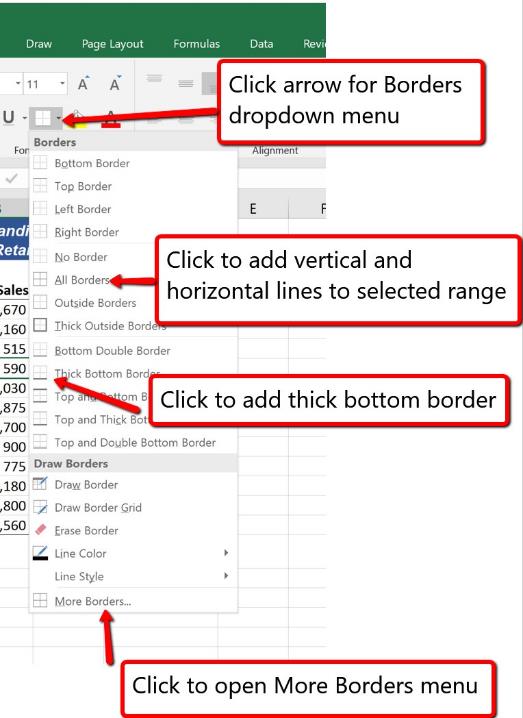
MedAttrib: Beginning to Intermediate Excel. MS Excel Borders Dropdown Menu.

Autowidth expansion

See how the column E for the salary data may be showing pound signs (####) in the data cells? This #### indicates that a numeric data column is too narrow to accommodate the data in it. While a text column will show some of the data in a too-narrow column (like the Address column), Excel can’t do this with numbers. Excel can’t do wrap text for numeric data, because numeric formats are usually for calculations, not just static text information.

You can fix this issue by widening the column. We’ll cover more column-related sizing later, but for now, the Autowidth action will suffice.

• Select the whole Column E – by clicking on the E column’s letter E at its top. Your cursor tip should then also show a down arrow.
• Slowly move your cursor to the right until the tip shows a Crosshair graphic. This means you have hovered over the border between columns E and F.
• Double-click while you see this crosshair, and column E should snap to a width that shows all the numbers within. You may have to try this a few times until you ‘get the hang of it’.

Text Effects

Alignment of cell content

The data you input into cells, unless formatted into some numeric form, likely defaults to a Bottom Alignment and to an Align Left. Any workbooks you inherit may change these defaults, and/or you may develop a different preference for your own work. For this worksheet, we’ll go for Top Alignment and Align Left. The file we are working with currently shows the first two columns are align center.

• Select cell A3, and click the Top Align button on the Home ribbon’s Alignment group.
• With A3 still selected, then click the Align Left button in the same Alignment group.

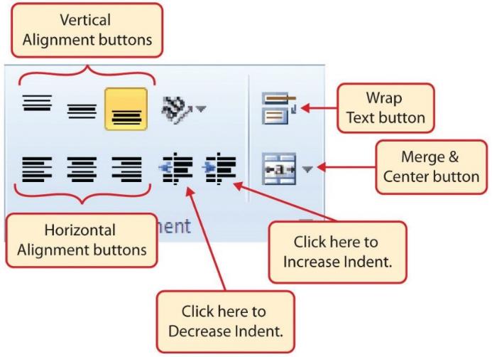
MedAttrib: Beginning to Intermediate Excel. MS Excel Alignment Group in Home Tab.

You can also change the alignments of several cells at one time:

• Select cells A4-A21.
• Click the Top Align and Align Left buttons again. The rest of the column should now look aligned like cell A3.
• Now, select cells B4-F21, and click the Top Align and Align Left buttons again. The rest of the table will also be formatted to be top aligned and aligned left.

There is just one cell that may remain unaligned properly: cell B3. Let’s use the Excel Format Painter button to fix that. The Format Painter button will pick up the formatting of a cell, and hold it until you click on another cell to ‘copy’ the format onto it.

• Select cell A3.
• Click once on the Format Painter ‘paintbrush’ button in the Home ribbon’s Clipboard group.
• Then, click once on cell B3. This should copy cell A3’s alignment format onto cell B3.
• SAVE your work as you go: the common keybind is CTRL S / Mac: CMD S.

Wrap text

Often, a text column may have not be wide enough for the information in it, and the text information will seem to be cut off. One way to fix this is to wrap text so that the cell will increase in size to accommodate the data and also push some of the data in what seems like a second (or more) line in the same cell.

• Select cell C4.
• Click on the Wrap Text button in the Home ribbon’s Font group. See how the row expands in height to show all the data which also now appears to be taking up a couple of “lines” of space inside the cell.
• Now, while cell C4 is still active, click on the Format Painter button from the Clipboard group.
• Then, while the Format Painter is active, hover then click over cells C5-C21 to apply the wrap text to the rest of the column.

Keyboard Shortcut: Wrap Text. Press ALT key and then letters H and W one at a time. MAC: N/A

Number Formatting

Text is easy to work with in Excel – the program just recognizes it as static data that is informational, not computational. However, numbers (unless used as dummy text in something like an address or phone number) are recognized as potential data to calculate. There are several types of numeric data that Excel recognizes, including:

• Comma, which adds a comma and a decimal point with a default 2 decimals after the decimal point.
• Dates, which offers both long and short US date formats.
• Time, which offers minutes and seconds.
• Percentage.
• Currency (discussed below).
• Accounting money (discussed below).
• Fraction.

For this example, let’s first format the Salary columns contents with a comma so that the numbers look like common ‘thousand’ units.

• Select cell E4.
• Look for the Home ribbon’s Number group, and click the arrow on its right side, which will show a dropdown selection of number formats.
• Scroll down that list until you find Currency, and click on that. The cell’s contents should now appear as $44,200.00.
• Let’s take out the “cents” part of that number. With cell E4 still active, click twice on the Number group’s Decrease Decimal. This should remove the .00 from the number.
• You can repeat the Currency format and Decrease Decimal steps after you select cells E5-E21.
  • Alternative method: use the Format Painter paintbrush to paint cell E4’s format over cells E5-E21. Click once on the Format Painter ‘paintbrush’ button in the Home ribbon’s Clipboard group while cell E4 is active, then paint over cells E5-E21.
• SAVE your work as you go: CTRL S / Mac CMD S.

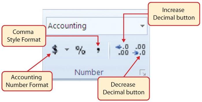
MedAttrib: Beginning to Intermediate Excel. MS Excel Number Group of Commands.

Formatting money standard practices

There are accepted professional formatting standards when spreadsheets contain only currency-related data. For this course, we will use the following Excel guidelines for formatting. The first image displays how to use Accounting number format when ALL figures are currency. Only the first row of data and the totals should be formatted with the Accounting format. The other data should be formatted with Comma style. There also needs to be a Top Border above the numbers in the total row. If any of the numbers have cents, you need to format all of the data with two decimal places.

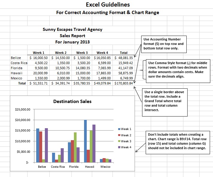
MedAttrib: Beginning to Intermediate Excel. MS Excel Accounting Standard format.

Often, an Excel spreadsheet will contain values that are both currency and non-currency in nature. When that is the case, you’ll want to use the guidelines in the following figure:

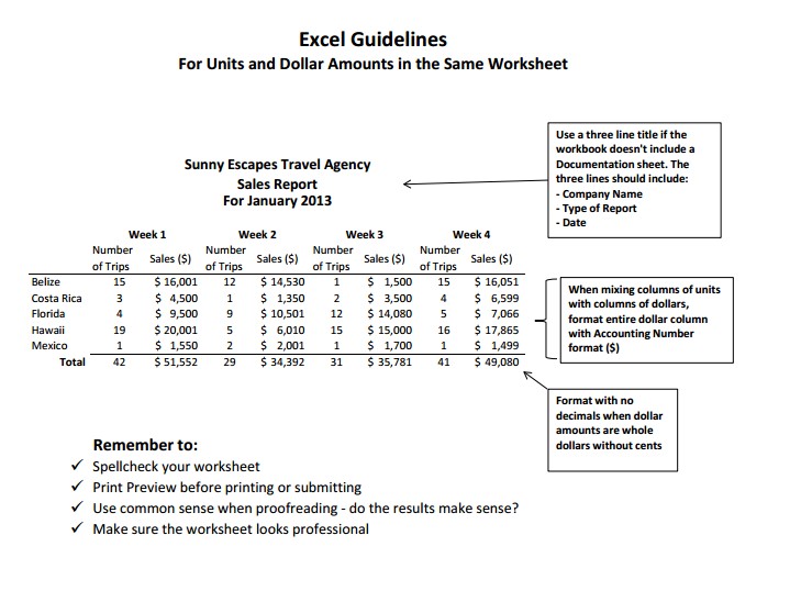
MedAttrib: Beginning to Intermediate Excel. MS Excel Currency/Mixed standard format.

The Format Cells panel

This was mentioned above. When you become proficient with Excel and the content you plan to produce, you can also use a more comprehensive Format Cells panel, which has several tabs you can choose from while formatting a cell or row or column.

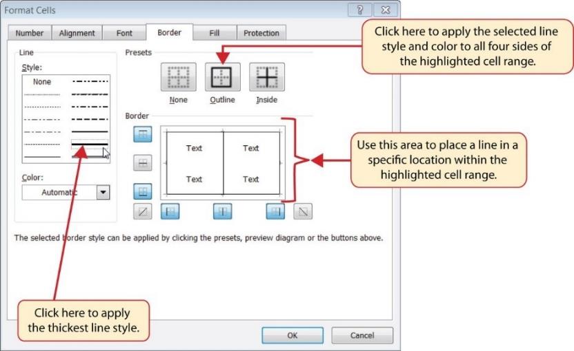
MedAttrib: Beginning to Intermediate Excel. MS Excel Borders Tab of Format Cells Dialog.

Here, we will add a line to the bottom of the data range we have been working on, so that you can input some data yourself, then format it. First, let’s add another line of data – about YOU.

• Click on cell A22, and type YOUR own first name in it.
• Add more information about yourself in cells B22-F22. Other than your own real last name, please feel comfortable ‘making up’ data for the other cells so that you preserve your confidentiality.
• Once you have your new data entered in row 22, click on cell A22.
• Then, in the Font group on the Home ribbon, look for a tiny Font settings arrow icon in the Font group’s lower right corner, and click on it. This should open the panel for Cell Formatting, which has 6 tabs in it: Number, Font, Alignment, Border, Fill, Protection.
• Since cell A22 is a static text data, you can use the Font and Alignment tabs to look at your choices and to change the cell’s format.
• Using the Alignment tab, make the contents of cell A22 top aligned and aligned left – if it is not already – then click Okay.
• Let’s try an other way. RIGHT-Click on cell B22, then scroll down the contextual menu until you see the Format Cells option (you may have to scroll down the menu list since it is near the bottom). Then, click on the Format Cells option. The same Format Cells panel you have already used will open.
• Using the Alignment tab, make the contents of cell B22 top aligned, aligned left if it is not already, then click OK.
  • Now, you can use either of these options to open the Cell Formatting panel as you adjust the formats of cells C22-F22.
• OR, you can just select cells of the row above your newly typed row – C21-F21 – and click the Format Painter paintbrush button on the ribbon, and then paint the style over cells C22-F22.
• SAVE your work as you go: CTRL S / Mac: CMD S.

Special formatting

Much of your data formatting will be basic tasks, like changing the color of the text or cell backgrounds, cell/column/row alignments and wrap, and selecting basic numeric formats like dates, accounting, percentages, etc. However, there are a number of basic additional formats that Excel lets you customize in cell formatting for more complicated needs, like:

• Phone numbers
• Social Security numbers
• Zip codes
• Showing negative numbers in stand-out formatting
• Additional date and time formats
• Additional fraction formats
• Customized number formats
• Validation techniques (later chapter)

These options are shown in the Format Cells panel, in the Number tab.

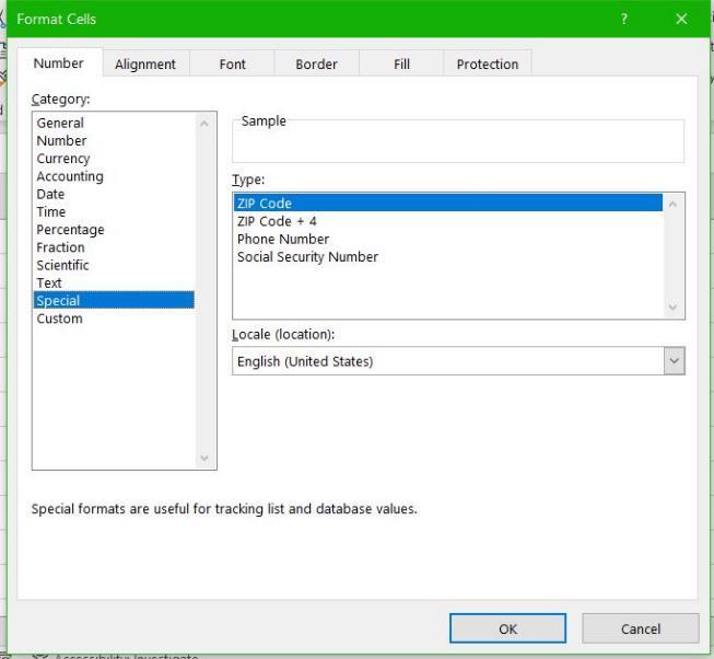
MedAttrib: autogenerated. MS Excel Format Cells panel.

Examples:

Phone number: 2065551234 = (206) 555-1234

Social Security Number: 2221111234 = 222-111-1234

Zip Code + 4: 981012345 = 98101-2345

Negative Number (one of the formats): -2700 = (2,700)

Sum Feature

Applying mathematical computations to a range of cells is accomplished through functions in Excel, which we will cover in detail in Part 4. However, the following steps will demonstrate how you can quickly sum the values in a column of data using the AutoSum command in the Home menu ribbon. It is now usually referred to as the Sum button but it automatically writes an addition formula for you.

• Click cell E23 in the worksheet.
• In the Home tab’s ribbon, look for the Editing group (more to the right side of the ribbon).
• Look for the button that looks like an and reads Sum when you hover over it. Click it while cell E23 is active.
• What you’ll ‘see’ in the Formula Bar: cell F23 will turn into a formula – =SUM(E4:E22) – and a dotted border and light blue fill will affect the column of numbers above it. This is Excel’s way of writing a basic addition calculation for you.
• When you press the ENTER key on your keyboard, the sum will calculate automatically, and add up the numbers in the column above cell E23.
• Now you will see the sum of the salaries of the people in the data range we have been working with, including the row you input about YOU!
• You should select the cell E23 again, and apply the Accounting format to it.
• SAVE your work as you go: CTRL S / Mac: CMD S.

We are finished with this activity!