Chapter 17: Functions – Financial

What We’ll Cover >>>

• Fundamentals of Loans
• PMT Function
• PPMT Function

In this chapter, we’ll work through a couple of basic financial functions in order to determine the payments and other conditions on a loan. Excel has a lot of financial functions, most of which are specialized to accounting and for loans, annuities, stocks, and other high-value skill areas. The loan-related functions are perhaps the simplest to use on a personal and general workplace support environment.

Fundamentals of Loans

A loan is a contractual agreement in which money is borrowed from a lender and paid back over a specific period of time. The amount of money that is borrowed from the lender is called the principal of the loan. The borrower is usually required to pay the principal of the loan plus interest. When you borrow money to buy a house, the loan is referred to as a mortgage. This is because the property being purchased also serves as collateral to ensure payment. In other words, the bank can take possession of your house if you fail to make loan payments.

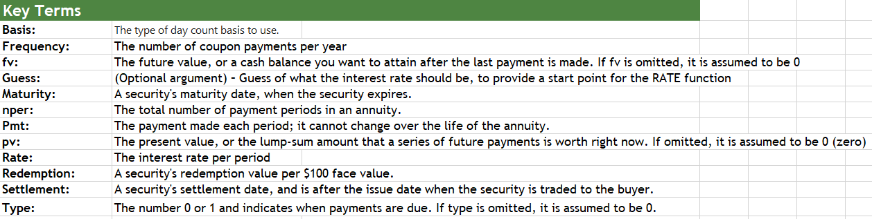
MedAttrib: author-generated. Table of loan terms.

A lender is required by law to provide borrowers with an amortization table when a loan contract is offered. Each time a payment is made on the loan, you are paying the bank an interest fee plus some of the loan principal. Each year the amount of interest paid to the bank decreases and the amount of money used to pay off the principal increases. This is because the bank is charging you interest on the amount of principal that has not been paid. As you pay off the principal, the interest rate is applied to a lower number, which reduces your interest charges.

PMT Function

The PMT function refers to payment. In Excel, loan payments are calculated through the PMT (payment) function. This function is more complex than the statistical functions covered in Section 2.2 “Statistical Functions”. With statistical functions, you are required to add only a range of cells or selected cells within the parentheses of the function, also known as the argument. With the PMT function, you must accurately define a series of arguments in order for the function to produce a reliable output.

Table 2.6 Arguments for the PMT Function

MedAttrib: author-generated. Table of PMT function arguments.

NOTE: by default, the result of the PMT function in Excel is shown as a negative number. This is because it represents an outgoing payment – something owed. To do this, you can place a negative sign between the equal sign and the function name PMT. Excel has other formats for negative numbers, like the number within parentheses, and/or the number shown in red.

When working with more complex functions such as the PMT, it is easiest to use the Function Dialog box. Use cell references for the arguments of the PMT function whenever possible. This will allow you the flexibility to change aspects of the loan and have the payment automatically recalculate.

ACTION: Try Me activity

We will work with a combination activities workbook, named Ch17-Finance.xlsx. Before you start working, go to your DataFiles folder and make a copy of the file for your Examples folder, then open that copy. Here is what we are aiming for. The red numbers in parentheses are one of Excel’s formats for negative (or in this case, owed) numbers.

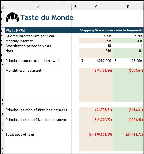
MedAttrib: author-generated. MS Excel loan activity.

The workbook has two sheets. The first is named LoanRepay, with a building loan, and a car loan. The second is an information sheet with a table of common financial functions you can use for your reference.

In the LoanRepay sheet, Taste du Monde has a loan for a shipping warehouse project, and a loan for a delivery vehicle.

The areas to be calculated are cells that have a background color:

• Light tan for the Warehouse loan in column C.
• Light green for the Vehicle loan in column D.

Let’s work on the warehouse loan first; it is the left-hand loan in the worksheet, ranging from cells C6 through C16.

The loan is for $2,250,000. It is for an expected 18 years (amortization). The interest it was taken for is 7.79%.

Our job is to determine the:

• Monthly loan payment
• Amount of loan principal the monthly payment is applied to at the beginning of the loan repayment (first month)
• Amount of loan principal the monthly payment is applied to at the end of the loan repayment (last month of 18 years)
• Total cost of the loan.

TIP: Comparable Arguments for PMT Function. When using functions such as PMT, make sure the arguments are defined in comparable terms. For example, if you are calculating the monthly payments of a loan, make sure both the Rate and Nper argument are expressed in terms of months. The function will produce an erroneous result if one argument is expressed in years while the other is expressed in months.

In calculating this data, we will have to calculate a few other things in order for the actual loan payment information to be able to be calculated correctly. This includes the:

• Monthly percentage rate of the annual interest rate (Monthly Interest)
• The number of months in the amortization period of 18 years (Nper)

This feels like a story problem. Ugh. Sorry.

Click on Cell C6. This is a simple calculation that doesn’t need the Function Arguments dialog, just a basic formula. This will give us the monthly interest rate from the annual one.

• In cell C6, type =C5/12
• AFTER you do this, change the data format of Cell C6 to Percentage using the Home Ribbon Number Group dropdown and choosing Percentage, then 2 decimal points.

Click on cell C8. This is also a simple calculation that doesn’t need the Function Arguments dialog. This will give us the number of months occurring in 18 years.

• In cell C8, type =C7*12

Now we have components to work on our PMT function. The cell F9 already provides the Pv (principle to be borrowed).

• Click on Cell C11 (for Monthly Loan Payment), and use the FX symbol to the left of the formula bar to open the Insert Function dialog box.
• In the search, type PMT and click GO.
• Select PMT and click OK.
• In the Function Arguments dialog box, add:
• Rate = cell C6
• Nper = cell C8
• Pv = Cell C9
• Ignore the Fv and the Type fields, since they are optional (you can tell because they are formatted in lighter gray).
• Click OK.

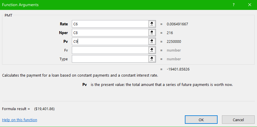
MedAttrib: author-generated. MS Excel Function Arguments dialog for PMT.

A number will populate Cell C11; it should be $19,401.86. This cell has already been formatted to show the number as a negative (a cost in repaying the loan, not revenue from a salary or bonus). This particular negative number format comes out as the number appearing in parentheses, and in red.

This is the monthly payment (PMT) for the loan under the terms of the interest and the 18 year repayment plan.

• SAVE your work.

PPMT Function

The PPMT function gives you the payment on the principal loan amount (Pv) for a given period, for an investment based on periodic constant payments and a constant interest rate. The principal amount will change over time, since the longer a loan is paid, the more of it will go to the principal and less to the interest.

In this activity, we’ll look at the payment on principal for the first month, then for the last month, of the 18-year loan period.

Click on cell C13. This is the very first month the loan will be paid, and most of the payment will apply to the interest. Our question is how much will be applied to the actual loan itself (the principal – Pv – of the $2,250,000)?

• Click on cell C13, and use the FX symbol to the left of the formula bar to open the Insert Function dialog box.
• In the search, type PPMT and click GO.
• Select PPMT and click OK.
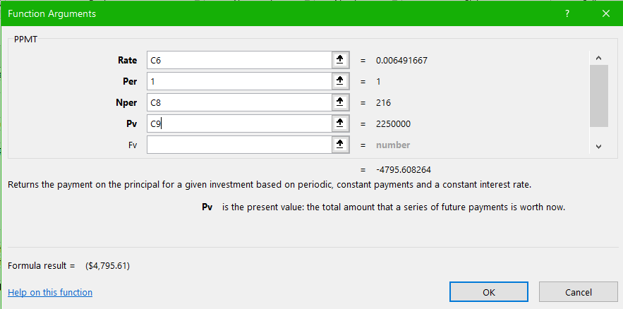
• In the Function Arguments dialog box, add:
• Rate = cell C6
• Per = 1
• Nper = cell C8
• Pv = cell C9
• Ignore the Fv field, since it is optional.
• Click OK.

A number will populate cell C13; it should be ($4,795.61) in red. This is how much of the monthly loan payment $19,401.86 (the Nper) in Month 1 (the Per) will be applied to the $2,250,000 (the Pv) loan amount; the rest will go to what is left of the interest.

MedAttrib: author-generated. MS Excel Function Arguments dialog for PPMT.

Now, let’s look at the same thing for the final month of the loan (month 216 from cell C8).

• Click on cell C14, and use the FX symbol to the left of the formula bar to open the Insert Function dialog box.
• In the search results select PPMT and click OK.
• In the Function Arguments dialog box, add:
• Rate = cell C6
• Per = 216
• Nper = cell C8
• Pv = Cell C9
• Ignore the Fv field, since it is optional.
• Click OK.

A number will populate cell C11; it should be ($19,276.72) in red. This is how much of the $19,401.86 (the Nper) in the final Month 216 (the Per) will be applied to the $2,250,000 (the Pv) loan amount. Most of it!

Now, let’s figure out how 18 years of paying the monthly loan will actually cost. We don’t need the Function Argument dialog for this; we are calculating the monthly loan payment by amortization years (18 years)

• Click on cell C16, and type =C11*C8

This is the monthly loan payment of $19,401.86 over 216 months (the nPer), and the total comes to a whopping ($4,190,801.39) in red.

• SAVE your work.

More Practice

Let’s find out if we get better terms and results for the delivery vehicle. It is the right-hand loan in the worksheet, ranging from Cells D6 through D16.

The loan is for $22,000. It is for an expected 4 years (amortization). The interest it was taken for is 5.20%.

• In cell D6, type =D5/12, then format the answer as Percentage with 2 decimal points)
• In cell D8 type =D7*12
• In cell D11, the formula – after using the Function Argument dialog – should come out as =PMT(D6,D8,D9)
• In cell D13, the formula, after using the Function Argument dialog, should come out as =PPMT(D6,1,D8,D9)
• In cell D14, you can practice calculating it based on what you learned from calculating cell C14 for the Warehouse loan.
• In cell D16, you can practice calculating it based on what you learned from calculating cell C16 for the Warehouse loan.
• SAVE your work. We’re finished!