Chapter 9: Table Creation

What We’ll Cover >>>

• Table Properties
• Table Design
• Table Object Creation
• Entering and Deleting Data
• Total Row

In Chapter 8, we got a taste of MS Excel tables when data imported from an Access Database and from a CSV file imported in the Excel table format. In this chapter, we will work on the result from Chapter 8. We previously worked with datasets, then discovered how simple sorts and filters needed extra attention to avoid corrupting the data.

However, Excel tables behave independently from the rest of the information on a worksheet. There are several advantages of Excel treating the data independently. For example, using integrated filters and sort functions you can effortlessly drill down data based on questions and in return get results. Excel will also automatically expand the table to accommodate new data entries and allows for automatic formatting, such as recoloring of banded rows or columns.

You will also notice Excel treats formulas and calculations differently in a table, showing structured column names, along with automatically filling a calculated field to the entire table or offering quick and easy table totaling tools. This is where naming your data range – in this case a table object – is efficient.

When graphing and charting table data we will also see Excel automatically adjusts off associated charts and ranges based on what the user is sorting or filtering at the time.

Table Properties

Turning a range of cells into an Excel table makes related data easier to analyze, visualize, and report. Structuring and planning table layouts are vital for data integrity. Below are guidelines to consider when designing and building a table from scratch. Your goal should be relating similar data so that summarizing and reporting out with graphs/charts makes sense. Table data should be easy to read. Tables that are expected to be bigger than the maximum column and row numbers for Excel should instead be stored in a database, then imported into Excel for calculations and analysis work.

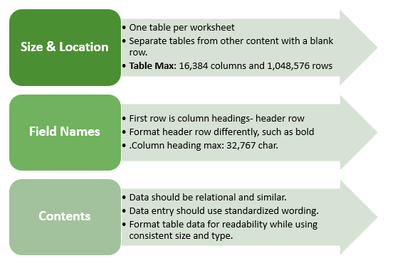
MedAttrib: author-generated. MS Excel Tables info.

Table Design

ACTION: Try Me activity

Let’s open the file Ch9-Tables.xlsx from the Datafiles folder. This is mostly the same result we had when we finished Chapter 8, but I deleted a bunch of customer rows to keep our work simple and streamlined. The Page Layout theme should already be the Office theme, which will give us the colors to use in this activity.

Here is what we are going to accomplish.

 

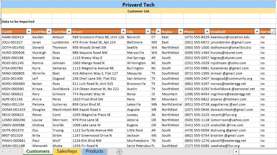
MedAttrib: author-generated. MS Excel finished Prisvard Tech customers table.

In the Ch9-Tables.xlsx file, we have three worksheets: Customers (orange tab), SalesReps (yellow tab) and Products (blue tab). The Customers and SalesReps sheets have an Excel table that was created when we imported data from an MS Access database. The Products sheet has a dataset that was imported from a CSV file then modified.

• Let’s work with the Customers table first. The Customers worksheet has blues, black, and yellows in the title and subtitle rows of the sheet. The table you imported may have appeared in any color in your Excel themes color palette. Mine came in as a table of green coloring. That sure doesn’t go with the Prisvard Tech theme of medium blues, yellow, black text, etc.
• Click anywhere in the Customers table.
• When you activate a table, a contextual Table Design tab ribbon opens near the top right of your Excel UI. Click on that tab.

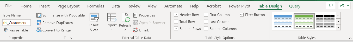
MedAttrib: author-generated. MS Excel Table Design ribbon.

The ribbon has several groups:

• Properties: Allows for naming and table resizing.
• Tools: Contains some table analysis tools.
• External Table Data: For use with linked live data sources, like a database that may have changes happen to it.
• Table Style Options: Basic table parts designation items.
• Table Styles: Color and layout styles for tables based on the Excel theme, color palette, and font palette you choose.
• For our purposes, we will use the groups of Properties, Table Style Options, and Table Styles.

Name a table

First, let’s name the table so that if it is ever used in a calculation, Excel can identify it more easily. Then we’ll change the table’s color design, then add a little more detail.

• With the table selected and active, look at the Table Design ribbon’s Properties group. The Table Name reads tbl_Customers. Let’s make this easier to use by overtyping with PTcustomers. This refers to Prisvard Tech customers.

Change Table Design

Next, let’s change the color scheme of the table to be an orange base to coordinate with the worksheet’s orange name tab.

• In the Table Styles, click the double-down arrow for a dropdown panel of table color options. In review, we should be using the default Office design theme for our color palette and font selections.
• In the Table Styles dropdown, choose the Orange, Table Style Medium, 17. This will change the table to a combination of a medium orange header row and light gray banded rows.

Let’s explore the table tools now. Notice the specific checkboxes to turn on table options, for example, you can choose to display banded rows or banded columns, or a total row etc. Currently, the Header Row, Banded Rows, and Filter Button selections are all turned on.

• Click on the table, and make sure the Table Design ribbon is active. Uncheck all three checkboxes that have a check, and look at what happens to the table.
• We clearly have a plain table without much visual definition, and no sorting or filtering capabilities. The Filter checkbox is grayed-out; the Excel table requires a header row to sort and filter information. Click to add a checkmark to the Header row checkbox.
• The Header row shows up again as orange, and the Filter button is also by default turned back on.
• Click the checkbox by First Column. Excel adds an orange fill to the whole of the table in Column A. Ugh. That is too hard on the eyes; uncheck that First Column checkbox.
• For visual definition, click the Banded Rows to add the gray bands again.
• SAVE your work as you go: Keybind is CTRL S / Mac CMD S.

Delete Table Columns

Before we move into the second worksheet for SalesReps, let’s do a little content cleanup of this Customer table. Part of this will include deleting a column or two and some other maintenance.

• Click in cell A10. Then click on the Home Tab, and look for the Cells group. In this group, click the Delete dropdown arrow, and from the list, choose Delete Table Columns. The ID column disappears.
• Let’s do the same for the Zip column in column G. Click anywhere in the Zip column in the table, then repeat the Home Tab, Cells group, Delete dropdown, Delete Tables Columns. the G column zip codes should disappear.

Fix Merge and Center conflict

Now, we have fewer columns, but the title and subtitle row of the worksheet are still shorter than the width of the table by one column. Let’s fix this. First, clink into cell A1, which is actually merged and centered across columns A – I.

• After clicking cell A1 which selects the merged cells, hold down the shift key and also click cell J1.
• Then, with seemingly all of A1-J1 selected, go to the Home ribbon’s Alignment group, and click the Merge and Center button once, then again.
• The first click will unmerge and uncenter Cells A1-I1, and the second click will merge and center all of Cells A1-J1.
• Repeat this task with row two to unmerge/uncenter cells A2-I2, and then merge and center cells A2-J2.

Tidy-up table data

• In Column H, which now has the Phone column, right-click on Cell H7. Choose Format Cells from the dropdown, and in the Format Cells panel’s Number tab, choose Special. In Special, select Phone Number, then click OK.
• Use the Home ribbon’s Clipboard group Format Painter to apply the style of cell H8 down through cell H101.
• Auto-resize the Column H phone numbers (or manually resize to about 12.5.)
• Auto-resize the Column I emails (or manually resize to about 24.)

Let’s sort the table so that we can modify a few of the email addresses to be hyperlinked.

• Click the Filter arrow in the Opt-In column J. Sort A-Z. This will sort by No and Yes responses.
• Select cell J7, and use Conditional Formatting for Highlight Cell Rules. The rule should be for equal to yes with the Yellow fill with dark yellow text.
• Then, use the format painter to paint that style over cells J8-J101. The last handful of responses – yes – will stand out.

These Yes opt-in responses need the email addresses in the column to their left to be hyperlinked. This is a manual task, but it is one worth practicing.

• Right-click on cell I87 which, assuming you sorted Column J so that the cells are at the top and Yes cells are at the bottom, should have the email lolombardo@lastname.com.
• Scroll down the menu from your Right-Click until you see Link, then click that. You should get an Insert Hyperlink dialog box.
• In Link To, select Existing File or Web Page.
• In the Text to Display, copy the contents, which should read lolombardo@lastname.com. Then, paste this email name to the Address field. Excel will automatically add a mailto: prefix to the pasted email address.
• Click OK. This will give you an active hyperlink.
• You can practice this a time or two, but the real answer to a situation with more than one or two links is to instead use a hyperlinking formula, which a more complex step for another chapter.
• SAVE your work as you go: Keybind is CTRL S / Mac CMD S.

ACTION: Quick Task

Let’s do a quick refresher of changing the Table Design with the second worksheet for SalesReps.

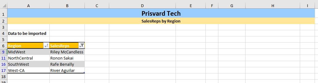
MedAttrib: author-generated. MS Excel Prisvard Tech salesreps table.

• In the SalesReps worksheet, click in the table of Regions / SalesReps.
• Go to the contextual Table Design tab, and use the Table Styles group to change the table design to Gold, Table Style Medium, 19. This gives us a gold bar header row that goes with the worksheet name tab’s yellow color. This one also has the gray banded rows in it.
• In the Table Design tab’s Properties group, overwrite tbl_SalesReps with PTregions.
• Right-click somewhere in the table’s A column. In the dropdown menu, choose Delete, then Table Columns. This should leave you with two columns.
• Auto-size the width of the two columns, which means that the content should not look cut off.
• Sort the Region column in order of A-Z using the table’s header row filter button.
• Use the header row filter button for the SalesReps column to filter with a text filter. Click the button, and in the dropdown, choose Text Filters, and in the flyout options, choose Begins With.
• In the Begins With field, type R then click OK.
• Now you can observe that the table shows only four sales rep names in alphabetical order of their regions.
• SAVE your work as you go: Keybind is CTRL S / Mac CMD S.

Table Creation

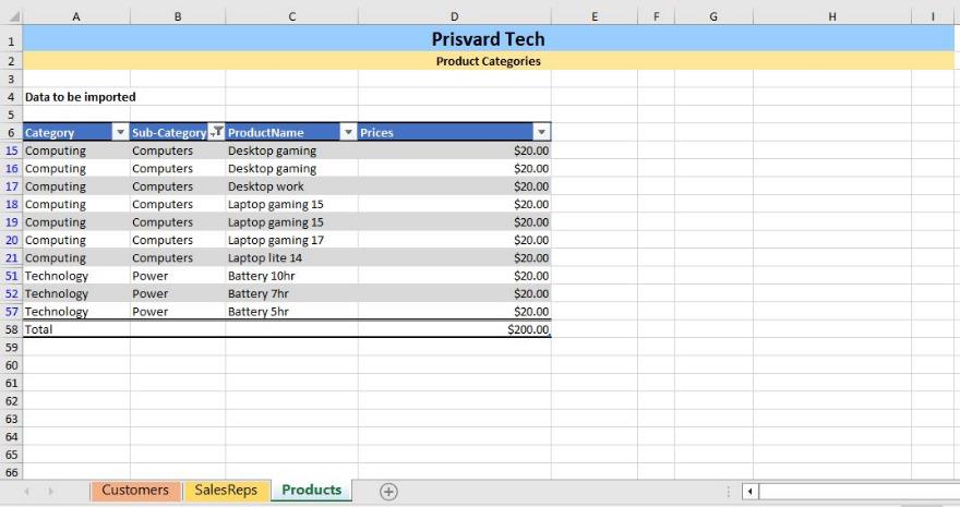
MedAttrib: author-generated. MS Excel Prisvard Tech products table.

In the Ch9-Tables.xlsx file, the third worksheet has a plain dataset. We need to convert this into an Excel table object – like those in the first two worksheets. Then we need to style it so that it follows the conventions of the rest of the workbook.

Click the Products worksheet tab which is the worksheet with the dataset. What do we see?

Right now, we see a dataset with a row that reads Column1, Column2, and Column3. The row below this reads Category, Sub-Category, and ProductName. If this data is going to make sense for later analysis, then row 6 needs to be deleted since Column1, 2, 3, etc. are not useful header names.

What we will be doing is converting the data range to an Excel Table object.

• Delete Row 6. Now, let’s make a table!
• Select the data in cells A6 – C56.
• With this range of data selected, go to the Insert ribbon, Tables group.
• In the Tables group, click the Table icon.
• A Create Table dialog box should open, which should already have entered the data range of cells you selected into the ‘Where is the data for your table?’ field. This should read:  $A$6:$C$56
• Click the checkbox next to My table has headers, then click OK.

The data range will now be encased in an Excel table. Now, let’s name the table, then change the table design.

• Click in the table, and then go to the Table Design ribbon. In it, overwrite the name Table1 with PTproducts.
• With the Design ribbon still active, use the Table Styles group to choose Blue Table Style Medium 16. This one has the gray banded rows in it.
• Adjust the width of the three table columns so that the content doesn’t overflow.
• SAVE your work.

Entering & Deleting Records

Tables require constant updating and may need calculations. When your table needs updating you can add/delete data, by adding/deleting rows, or columns. Excel adjusts the table automatically to the new content if you add it to a row or column after an existing one. The format applied to the banded rows updates to accommodate the new data set size.

When calculations are needed you can create a calculated column or use the built-in Total Row tool. Excel tables are a fantastic tool for entering formulas efficiently in a calculated column. Excel allows you to enter a single formula in one cell, and then that formula will automatically expand to the rest of the column by itself. There’s no need to use the Fill or Copy commands. This feature can be incredibly time-saving, especially if you have a lot of rows. And the same thing happens when you change a formula; the change will also expand to the rest of the calculated column.

For now, we’ll just add a little data.

In the Ch9-Tables.xlsx file, we’ll work more on the 3^rd worksheet: Products. Currently, the table ends at row 56.

• Click into Cell A57, and type the word Technology, then click your keyboard’s Tab button.
• In the next cell, type Power, then click Tab again.
• In the third cell, type Battery 5hr then hit Enter. The table should have automatically expanded its format and range down to accommodate the new row of text you entered.

TIP: Adding Rows. It can be tempting to insert blank rows further up in a table and add data, yet with the ease of sorting and filtering, that isn’t really an efficient way of adding data.

Next, let’s add a column. We’ll want to add some pricing information for the Products. We’ll just do the simple thing and add a repeating default price so that we can move quickly.

• Click in cell D6, which is to the right of the 3^rd header column title.
• Type Prices then click your Enter key. Whoa! Excel just added a whole column of formatted space to our table. Cool.
• In cell D7, type 20, then press Enter.
• Click on cell D7, then use the Home ribbon Numbers group, and choose Currency. The Cell should show $20.00.
• Copy the contents of Cell D7, and paste the data into cells D8 – D57.

Why did we do this? We want to add a total row to the table using the Table Design tab options. A total row needs something to total.

Total Row

A useful table tool for quick data analysis is the Total Row. You can quickly total data in an Excel table by enabling the Total Row option, and then use one of several built-in functions provided in a drop-down list, per column. The Total row, which is added to the end of the table after the last data record, can calculate summary statistics, including the average, sum, minimum, and maximum of select fields within the table.

The Total row is formatted with values displayed in bold, the double border line option is separating the data records from the Total row.

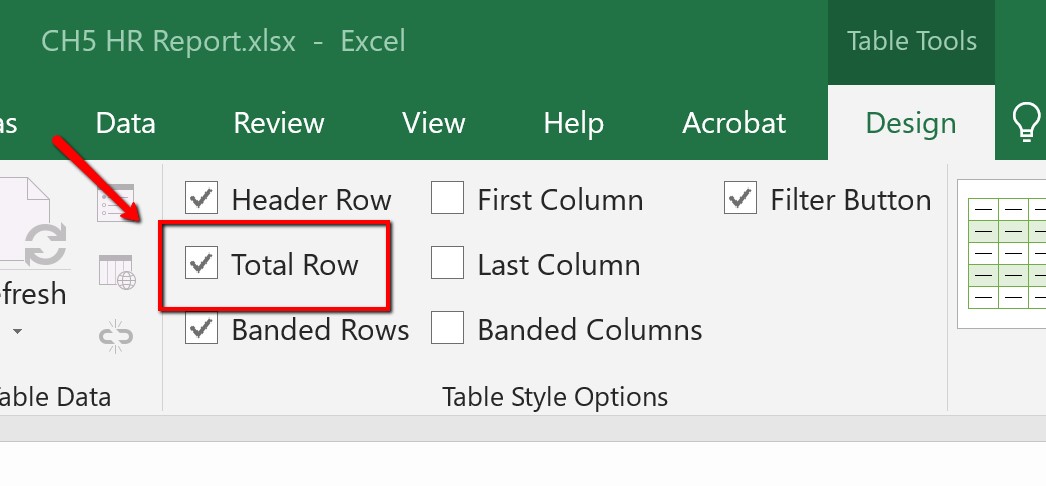
MedAttrib: Beginning to Intermediate Excel. MS Excel total row.

• Click anywhere in the Products table, then choose the Table Design ribbon.
• In the Table Design, click the Total Row checkbox in the Table Style Options group. This will add a table Total Row.
• Excel redirects you to the bottom of the table to view the total row, where a SUM was just calculated by default in the Prices column.

Before we close this activity, let’s filter the Products table for only computers and power products.

• Click anywhere in the Products table.
• Filter the Sub-Category column with the Filter button by opening the dropdown filter options.
• In the options, uncheck the box for Select All.
• Then check the checkboxes for only Computer and Power. The table will then “collapse” rows to show only the Computer and Power sub-category products, and the total for only those products.
• SAVE your work, then close the file. We’re done!