Chapter 5: Inserts and Visual Appeal

What We’ll Cover >>>

• Themes
• Modifying Themes
• Tables
• WordArt
• Pictures
• Icons
• SmartArt
• Hyperlinks

Excel is primarily a spreadsheet for computations and data analysis. However, it also has a number of basic visual communication enhancements, like Microsoft® Word® and Microsoft® PowerPoint®. This is mainly so that documents shared by the same entity, like a business or a multi-application project can use the same stylistic elements between them. In this chapter, we will work with a small file and play around with adding elements to it.

ACTION: Try Me activity

For this chapter, we will use the data file Ch5-Inserts.xlsx in order to demonstrate the various steps. Please find and open Ch5-Inserts.xlsx, and save a copy to your Examples folder. Most of our work will use the Inserts menu ribbon, with some coverage of the Page Layout menu ribbon for only themes, colors, fonts, and effects.

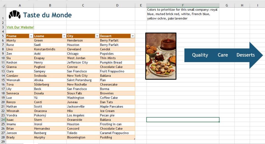
MedAttrib: author-generated. MS Excel Ch5-Inserts.xlsx final result. Dessert: Creative Commons

Themes

We’ll start with the Page Layout ribbon. This is because when putting together a document or spreadsheet, it can be more efficient to look from the macro level to the granular level; the theme, colors, and other things that affect all the styling of the worksheet should be considered when creating the project, so that any inserts, tables, and charts/graphs flow from the color and font selections.

In Ch5-Inserts.xlsx, we’ll change the theme first, then determine if it meets our needs and how to adjust it by choosing other colors and/or fonts. Normally, Excel defaults to the current Office theme, which gives a palette of colors and shades from across the color spectrum. However, on spreadsheets, you may instead prefer a different color set, or inherit a workbook at work that uses another color scheme, or be tasked with an assignment with certain theme specifications. While Excel is designed for themes to be changed almost effortlessly and without technical glitching, it is always good to plan your work and do steps efficiently to avoid rework or conflicts to very large spreadsheets later.

Colors to prioritize for this small company: royal blue, muted brick red, white, French blue, yellow ochre, pale lavender. We’ll find out what applies in the color themes, if any. Blues and related muted colors are preferred. We may not find them all in a theme, but a theme that captures several will work.

Note that the file you open already has a deep blueish color applied to the data range’s header row, which will be important to remember later. The text in the row seems invisible as a result.

• Click on cell A1, then choose the Page Layout menu ribbon.
• In the Themes group of the ribbon, choose the Themes dropdown box arrow.
• For fun, just click on a few – on your screen outside the Themes dropdown, you can see the fonts and the header row color seems to Preview a change.
• We’ll settle on the Berlin theme, because the font selection seems easy enough to read with a little added text boldness, but not too stylistic to make a workbook hard to understand.
• The existing color of the header row will have changed color.
• SAVE your work as you go: Keybind is CTRL S / Mac CMD S.

Note: this course is focusing on Excel for Windows (PC) and the assumption that your full installation has all the built-in items, like themes, color palettes, etc. However. If you don’t have some of these themes or named palettes / font collections (like with a Mac), choose what you can that seems closest to gain the skills-building anyway.

Modifying Themes

Now, the Berlin theme has great fonts, but the color palette may not work. Let’s check it out. The Taste du Monde header row is currently kind of a orange-brown color. Not good for the company’s planned color scheme.

• Right-click on the Cell A5, the first cell in the header row, which will pull up a menu list.
• Choose the Format Cells (you may have to scroll down the menu list since it is near the bottom), which opens the Format Cells panel. In this panel, choose the Fill tab.
• In the Fill tab, look at the upper left that shows a palette of 10 columns of colors and their shades. This is the color palette for this particular theme, and includes maybe a couple of the muted French county colors we could use, but no blues. No thank you!
• Exit the Format Cells panel by clicking Cancel.
• SAVE your work as you go: Keybind is CTRL S / Mac CMD S.

Colors Palette

Now, let’s consider other color options for this theme. While keeping the Berlin theme, we will use the Colors panel to look at options.

• You can click anywhere on the work area of your worksheet; then In the Themes group of the ribbon, choose the Colors dropdown box arrow.
• We are looking for something that has a dark blue, medium blue, darkish brick red, and a couple of neutral colors in the palette that could be purposed for Taste du Monde. Scroll down the Colors dropdown, and notice how our header row’s color changes. The closest we may find is the Aspect color palette.
• In the Colors palette, choose Aspect (near or at the bottom of the list). This looks mostly like reds and so we’ll repeat looking at cell A5 in the Cell Format panel’s Fill Tab to check out the color palette’s spread of colors.
• In the Cell Format panel’s Fill Tab, look at the color palette. In it, there is a blue column with a dark blue and a French blue, dark brick reddish color, a lavender color, a kind of light tan, and white. This should do.

Fonts Palette

We can look at the Fonts palette to determine if we want a different font set.

• You can click anywhere on the work area of your worksheet; then In the Themes group of the ribbon, choose the Fonts dropdown box arrow.
• In the dropdown list, there are a number of font sets. Unfortunately, the dropdown list does not show which specific font set we are using. You need to click on one of the cells in your workspace to see, in the Home ribbon’s Font Field which font this document is using: Trebuchet.
• Scroll down and see how the fonts on your worksheet seem affected in the preview. You can choose to experiment by clicking on one or two, but for Taste du Monde, we’ll stay with the Berlin theme’s chosen fonts.
• SAVE your work as you go: Keybind is CTRL S / Mac CMD S.

Effects Panel

The Effects panel lets you preview some effects that can be used on graphics like shapes, SmartArt, WordArt, and image borders in Excel workbooks. We don’t have a shape inserted yet, but we can change this effect in advance. We may see how this is reflected in a later inserted item.

• In the Themes group of the ribbon, choose the Effects dropdown box arrow.
• Click on the Glossy effect to choose it.
• Note: Effects can be very subtle, depending on the theme used. Some themes will show more effects, and others, like Berlin, may not show much effect detail at all.

Tables

Tables are an Excel mainstay of ‘collecting’ data in an integrated format. They allow the data rows and columns to be seamlessly connected to each other for efficient sorting, filtering, styling, and calculations. We will cover tables in detail in Part 2. However, for this activity, we want to convert the data range of cells A5 through D28 from a plain data range to an Excel Table object, because this is something that can be better modified with the Theme and Color Palette’s options.

Now, we will cover the Inserts menu ribbon options. For the purpose of this chapter in Inserts, we will simply ‘insert’ a table for the practice, since it is a very important skill. Inserting a table over a range of data (bunch of cells) actually converts the existing cells to the table object, it doesn’t put in a new separate table,

• Click on cell A5.
• Go to the Inserts menu ribbon, to the Tables group.
• Click on the Table button.
• When a small Create Table dialog box opens, put a checkmark in the My table has headers field.
• Look over the field for “Where is the data for your table.” Excel has improved significantly over its versions, so that the program can discern a collection of data in a range of cells next to each other (columns, rows). As a result, the field for Where is the data… should already be populated with the information $A$5:$D$28, which is the spread of cells from the first cell in the Header row to the final cell at the lower left of the range of data.
• If, for some reason, you do not see this info in the data range field, you can manually type it in: $A$5:$D$28
• Click the OK button on the Create Table dialog box. The range of data from A5-D28 will have converted the plain data range into a default table format with filters and banded color rows that uses the Berlin theme’s fonts and the color palette we chose.
• One more thing: we will want the table’s header row text to be white, so you need to select the header row cells and change the font color to white so you can see the text in the colored background.
• For now, we will do no more work with this table. Lots more on tables will be in Part 2!
• SAVE your work.

WordArt

WordArt lets you add a special stylized and editable text graphic. In Excel, graphics like WordArt, SmartArt, images, and shapes are all ‘unanchored’ to cells, which means that they float above cells and can be easily moved without affecting the data inside your cells. We won’t cover the other Text Group button options in this activity, but they work much the same way as the WordArt one.

Here is a refresher of what the final project should look like.

• Delete the content in cell A1.
• In the Inserts menu ribbon, click the Text group button for Text, and select WordArt from the dropdown menu.
• In WordArt, click the last option on the second row: Fill: Dark blue Accent Color 3; Sharp Bevel
• A WordArt box will appear on your workspace. It is in a poor position and the text seems really big. The good news is that this is editable.
• First, click inside the WordArt. This ‘activates’ the WordArt, and a new, contextual ribbon appears at the right-hand side of your Menu bar, called Shape Format.

This same kind of contextual ribbon options shows up for anything you can insert in Excel. For now, we won’t work with this one. Instead:

• Type over the words in the WordArt to replace them with Taste du Monde.
• Next, select all those words, and using your Home ribbon’s font size field, choose the font size 24.
• Then, click outside the WordArt box, carefully hover your mouse cursor over it until you get a dark crosshairs icon, and press down to select the WordArt box for movement.
• Move it by dragging the box over to the right border of cell B1.
• SAVE your work.

Pictures

Excel lets you add illustrations, like photos and clipart. Like WordArt, pictures are ‘unanchored’ to cells, which means that they float above cells and can be easily moved without affecting the data inside your cells. Also, like WordArt, an inserted picture (when made active by clicking on it) will reveal a contextual Menu ribbon for doing editing work on the inserted item.

• In the Inserts menu ribbon, click the Illustrations group button for Pictures.
• Click Pictures, which shows you image locations to choose from: This Device, or Stock Images, or Online Pictures.
• In this case, assuming you are online, choose the Online Pictures option, which will pull open an Online Pictures window only.
• If you see the option in this window, place a checkmark in the Creative Commons Only checkbox, so that you use only freely available images.
• Then, type in YOUR favorite type of dessert – if you have one – and look at the results you get. Then, choose one of the images and click it, which will insert it into your worksheet.

Your image could insert itself  in any size, so we’ll set a size for whatever image we use so that it works nicely in the Taste du Monde worksheet.

• Click your inserted picture. This ‘activates’ the picture so that a new, contextual ribbon appears at the right-hand side of your Menu/Ribbon bar, called Picture Format. We will use this ribbon for the next several steps.
• In the Picture Format ribbon, on the far right, choose the text field for the horizontal size, and type in 1.5.” This will resize your picture to 1.5 inches wide, and to whatever the proportional height is.
• Next, click the Accessibility button on the Accessibility group. In the text field, type “image of my favorite dessert,” and place a checkmark in the Mark as decorative checkbox. This allows Excel to consider this image as accessible in the program.
• Then, in the Picture Styles group, choose Picture Border, and in the dropdown, choose the color black. This adds a very narrow border to your picture.
• in the Picture Styles group, choose Picture Border again, and in the dropdown, choose Weight, and on the flyout menu, choose 3pt. This will make a more prominent border for your picture.
• Drag the picture so that it floats just to the top right edge of the Taste du Monde table, like in the final example above.
• SAVE your work.

The Picture Format menu ribbon offers all sorts of options for you to work with:

• Adjustments like color correction, colorizing, and artistic effects;
• Picture Styles like preset borders and Picture borders / effects / layout;
• Arrange options like Bringing Forward and Sending Back; and
• Size options like Crop and resizing fields.
• Just for fun, you could try using an artistic effect on the image.
• Note: Even though we selected “frosted” in the Effects Panel selection above, this effect may not actually appear prominently on an image – it will usually appear for inserting shapes and such. No worries!

Icons

Excel also lets you add other illustrations, like icons. Icons are built into the Excel subscription and Excel accesses them online. Icons also are ‘unanchored’ to cells, and an inserted active icon will reveal a contextual Menu ribbon for doing editing work on the inserted item.

• In the Inserts ribbon, click the Illustrations group button for Icons.
• Excel will open a Stock Images online search panel in the Microsoft® library for Excel/Office subscribers. This search area has tabs for Images, Icons, Cutout People, Stickers, Illustrations, and Cartoons that are in the Microsoft® library.
• In the Icon tab of the Stock Images search, type food, then scroll down until you see a little black croissant. You could also type “croissant” in the search bar.
• Click the selector circle at the top right of the croissant icon, then click the Insert button at the bottom right of the Stock Images search panel.
• The icon will appear in your Excel workspace, floating somewhere in the center. Clicking on it will activate a Graphics Format contextual menu ribbon.
• You can manually resize the icon by dragging the lower right-hand corner inwards to make it a little smaller, say .7 inches. Or you can click on the icon and type .7” in the Graphics Format ribbon.
• Then, drag the croissant icon over to the left side of Cell A1, like in our example final image above.
• After that, click on and drag the WordArt of Taste du Monde a little to the left so that it aligns with the croissant icon, like in our example final image above.
• SAVE your work.

SmartArt

SmartArt is a Microsoft illustration that combines editable linked shapes with text boxes, and allows you to an alternate way of structuring visual communication information. SmartArt is ‘unanchored’ to cells, and an inserted active SmartArt item will reveal a contextual Menu ribbon for doing editing work on the inserted item.

• In the Inserts ribbon, click the Illustrations group button and look for the SmartArt button.
• Excel will open a SmartArt panel that offers many SmartArt choices in several group options.
• From the top group option – All – scroll down and choose the Continuous Arrow Process, then click OK.

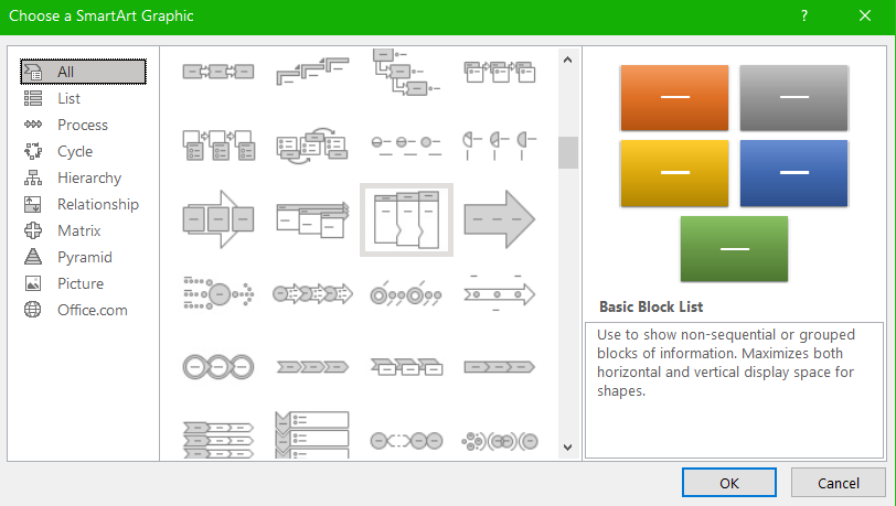
MedAttrib: author-generated. MS Excel SmartArt panel.

• The SmartArt will appear in your Excel workspace, floating somewhere in the center. Clicking on it will activate a SmartArt Design contextual menu ribbon and another contextual ribbon to its left simply called Format.
• In the SmartArt Design ribbon, let’s change the color using the SmartArt Styles group. Choose Accent 3, which is the dark blue.
• Inside the SmartArt, click the first Text field and type Quality. Click in the second Text field and type Care. Click in the second Text field and type Desserts.
• Inside the SmartArt, click on the Format contextual ribbon. In the ribbon’s WordArt styles, click on the Text Fill button. In the Text Fill palette, choose White.
• Do these same steps to change the words Quality and Desserts to white.
• Click on the border of the SmartArt image, and in the Format ribbon’s right side, choose Size. In Size / Width, type 4”.
• Carefully drag the whole SmartArt graphic so that it flies out about ½ inch from the right side of your image of a dessert.
• SAVE your work.

SmartArt has a lot of options to work with, especially in changing colors, effects, adding text and levels, and more. There are also several types of SmartArt groups:

• List: Non-sequential information
• Process: Steps in a process/timeline
• Cycle: Illustrate a continual process
• Hierarchy: Organization chart or decision tree
• Relationship: Show connections
• Matrix: Demonstrate how parts relate to the whole.
• Pictures: use to accent content.
• Pyramid: Illustrate proportional relationships.

In SmartArt, you can add and organize text in hierarchical levels either manually or with a text pane. There is too much to cover when our focus is on Excel, so it is recommended that you experiment on your own for this.

Hyperlinks

You may need to add hyperlinks in Excel worksheets, especially if you create/maintain lists of customers with email addresses, and companies with website locations.

• Select Cell A3, which reads Visit Our Website!
• In the Inserts ribbon, click the Hyperlink button (near the middle right). There may be a list of recent documents you have used, but ignore those for now; click Insert Link which is listed at the bottom of the dropdown.

Insert Link will open an Insert Hyperlink panel, which offers the options to link to: an existing file or web page, a place in the same workbook, a new creation of another document, or an email address.

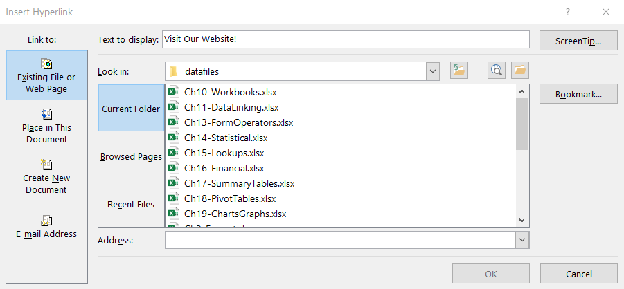
MedAttrib: author-generated. MS Excel Insert hyperlinks.

• Choose the Existing File or Web Page option.
• Then, in the Address field at the bottom of the panel, type: http://www.tastedumonde.biz (Note: this is a made-up address for this task; to my knowledge no such business actually exists).
• SAVE your work, then close your file. We’re done with it!

Keyboard Shortcut: Add Hyperlink. Hold down CTRL key while pressing letter K on your keyboard / Mac CMD K.