Chapter 12: Data Linking

What We’ll Cover >>>

• Data Linking Formula
• Click-Linking
• Linking Between Workbooks

An additional way to get data from one place to another is to use a Cell-linking method. This is when a workbook cell references data from another cell in a way that copies it in and also links it to the original cell. For instance, a master sheet may be updated, and have several other sheets dependent on it. If the original data is manually added to each worksheet, then new changes need to also be manually updated on each worksheet. Sigh.

However, if data is entered into one worksheet, and cells in one or more locations on other worksheets need that data, Cell-Linking to that data will bring it in. And, the only place the data needs to be updated is in the original sheet that the other sheets have linked to. Change that data – such as correcting a spelling or changing a date, and that data will automatically change on the other sheets referencing that data as well. Cool, huh?

ACTION: Try Me activity

We will work with Ihoosha Online Training again. In this case, we will work on the Ch12–DataLinking.xlsx file, and we will also need to reference the Ch12–DLSupport.xlsx file. You should make a copy of these from your DataFiles folder and put them into your Examples folder so you can work on the copies.

Open the Ch12–DataLinking.xlsx file from your and look it over. There are four sheets: MarchLeads, 2023Students, GraphicsClass, and 2022Fees.

Data Linking Formula

The Data linking method is as simple as telling a cell where to get data from. We can do that using a simple Excel formula method. The first thing we want to do is to add the leads from the MarchLeads sheet (host) to the end of the 2023Students sheet’s table (already populated).

Enter the 2023Students sheet. The dataset in here is not an actual Excel table object, because this can have trouble adding rows of new data into the table object structure we will be applying here. Data needs to be added, then we can create an Excel table object.

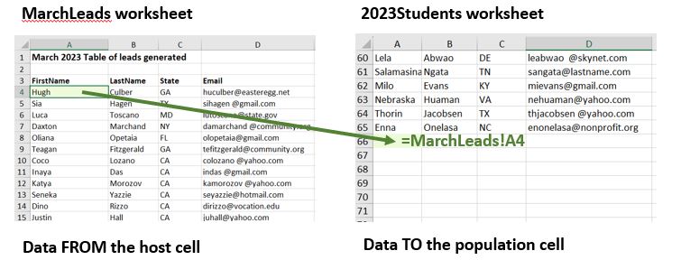
MedAttrib: author-generated. MS Excel data-linking process.

In 2023Students, click on Cell A66. We need to tell that cell where to find some data. The cell is at the bottom of a column of student first names, and we want to add another first name of a student – which happens to be in the MarchLeads worksheet.

• Now, in Cell A66, type this specific formula: =MarchLeads!A4 then press your enter button. This should bring in the first student’s First Name from the worksheet called MarchLeads cell A4. That name is Hugh.
• In cell B66, again type the linking formula, this time for the MarchLead sheet’s first student’s LastName. The formula is =MarchLeads!B4 then press enter, which populates the 2023Student worksheet’s cell B66 with the last name Culber.
• In the 2023Student worksheet’s cell C66, type =MarchLeads!C4 and press enter.
• In 2023Student worksheet’s cell D66, type =MarchLeads!D4 and press enter.

Now you should see one record of a new student, which was “imported” / linked – in from the host MarchLeads sheet to the bottom of the already populated 2023Students sheet. Let’s make a change to see why this is useful.

• Enter the MarchLeads worksheetsheet, and go to Cell B4. We have the incorrect last name, which should be Colbert. Overwrite the name Culber with Colbert.
• Enter the 2023Students sheet, and look at cell B66. The change we made in the other worksheet is also updated here: Culver changed to Colbert.
• SAVE your work.

Data Click-Linking

There is an even easier way that doesn’t require you to type that little formula, and it is a little more accurate, especially when typing can bring in errors. (Your instructor has typing butterfingers).

• In the 2023Students sheet, click in cell A67.
• In cell A67, type only the equals sign: =
• Then, while still in the cell, enter the MarchLeads worksheet, and find cell A5, and CLICK on that cell. Excel will automatically finish the formula with the cell’s address (which is MarchLeads!A5) and link the cells.
• In the 2023Students sheet, click in cell B67. Then enter the MarchLeads sheet, and find cell B5, and CLICK on that cell.
• In the 2023Students sheet, click in cell C67. Then enter the MarchLeads sheet, and find cell C5, and CLICK on that cell.
• In the 2023Students sheet, click in cell D67. Then enter the MarchLeads sheet, and find cell D5, and CLICK on that cell.
• SAVE your work.

ANNNND now, you are asking “Are we there yet??” Almost, yes. Because, we now get to apply the formulas to the cells below the ones we just input.

• In the 2023Students sheet, click cell A67 and copy it. Then, paste it down to  cell A68.
• Check the formula in Cell A68. It should read =MarchLeads!A6.

Given that there are 47 more first names in the MarchLeads sheet, you can safely copy the contents of Cell A68 down 47 more cells in Column A, from cell A69 – cell A115. All the relevant student first names from the MarchLeads sheet column A will populate the 2023Students sheet column A. Let’s try.

• In the 2023Students worksheet, copy cell A68, and paste it into cells A69 – A115.

I think I can guess what you are thinking. It is either time to go hydrate with your favorite beverage, or you can try this fast linking in an even more efficient way.

• In the 2023Students sheet, select all three cells B67, C67, and D67, and copy them.
• Place your cursor at cell B68, and select all the cells from B68 – D115, then Paste using either CTRL / CMD V (Mac), or the Home tab’s Clipboard group’s Paste icon.
• WHOOSH! All those cells should populate with the click-linked formula for you.
• Are we THERE yet?
• Yes.
• SAVE your work.

You should see that all the student last names, states, and email addresses from the MarchLeads sheet have now populated the 2023Students sheet Columns B through D.

One more important thing: This click linking is good to keep active in the populated worksheet if you plan to make minor data changes in the host sheet. However, this means that if the order of the data in the MarchLeads sheet changes, like if that sheet is sorted, the data references in the 2023Students sheet will repopulate with the new data from the host sheet. In a small spreadsheet, this might not be a real issue. However, imagine a sheet with hundreds of click-linked rows of data suddenly had massive changes in the data, especially if other data in the records did not change with it.

If you are at all concerned about your populated data getting changed on you, you can “break” the link easily, while keeping the data you just click-linked in. Let’s do that here.

• In the 2023Students sheet, select all the data from Cells A66 – D115.
• Copy all the data in that selection, then Paste VALUES of the data over itself ( the same cells A66 – D115).
• Using the Home tab’s Clipboard group’s Paste icon, click the down arrow for the dropdown paste options menu, and choose Paste VALUES.
• Then, click in cell A66, which had the click-link value, and you can observe that it no longer has the formula, just the results. The data is safe from any changes, resorts, filters, or other big changes that could happen in the MarchLeads worksheet.

Let’s do a bit more work with this particular sheet, to clean things up.

• Click anywhere in your 2023Students sheet, then use Insert to convert the dataset into an Excel table object with headers.
• Use the Table Design tab’s Table Styles group to select the Turquoise Table Style Light 10 to apply it to the table.
• In the Table Design tab, click the checkbox for Total Row.
• Scroll to the bottom of the table, so that you can see the total row below the final student LastName.
• Click in cell B116, and you should see a filter down arrow. Click it, and choose Count. This gives the count of students listed in the table.
• Now, go up the worksheet to cell F3. In the cell, type the equal sign = then click in cell B116 and press Enter. The number 110 appears in cell F3.
• SAVE your work.

This is a really useful way of grabbing a lot of data from one place and bringing it over to another. Let’s practice it a little more. We’ll populate the GraphicsClass worksheet with information from the 2023Students worksheet.

• In the GraphicsClass worksheet, click on cell B6. In it, type = then click on one of the cells in the 2023Students worksheet that shows the Comp203 course, like in the record for Sonora Vargas. In my sheet, that is cell F50.
• In the GraphicsClass worksheet, click on cell B7. In it, type = then click the 2023Students cell G50.
• In the GraphicsClass worksheet, click on cell B8. In it, type = then click the 2023Students cell H50.

If you would like, you can use the rest of the GraphicsClass worksheet to practice populating the class with names from records in the 2023Students worksheet of students who are taking the Comp203 – Graphics Suite course.

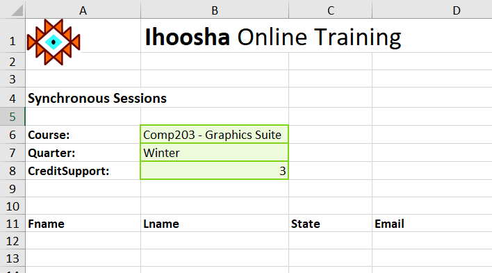
MedAttrib: author-generated. More click-linking.

Linking Between Workbooks

Another way to get data is to use a similar process but with an external workbook. This isn’t quite like importing from a database, though it is a little more complex than the click-linking we have been doing here.

You need to have easy access to the file you want to link to for accessing the specific data. And, the file should be saved into the directory you link from, because if the file is moved, the links could break the current spreadsheet.

In our case, we will use the other Chapter 12 file you hopefully also put into your working folder: Ch12–DLSupport.xlsx.

Look at the currently open Ch12–DataLinking.xlsx file, for the 2022Fees worksheet. That worksheet only needs two pieces of information, likely from a 2022 file: the total number of students, and the total amount of fees.

• Open the Ch12–DLSupport.xlsx file. There is only one worksheet. Scroll to the bottom so that you can access row 167, where there is a count of student last names and a currency number.
• In the Ch12–DataLinking.xlsx file’s 2022Fees worksheet, Click cell C5, then type =
• Then, navigate to the Ch12–DLSupport.xlsx file, and click in cell C167 and press your Enter button. Excel will immediately return to cell C5 in the 2022Fees worksheet, and display the count in it.
• Now, In the Ch12–DataLinking.xlsx file’s 2022Fees worksheet, Click cell C6, then type =
• Then, navigate back to the Ch12–DLSupport.xlsx file, and click in cell H167 and press your Enter button. Excel will immediately return to cell C6 in the 2022Fees worksheet, and display the currency amount in it.
• Close the Ch12–DLSupport.xlsx file without saving it so that only your 2022Fees worksheet is still open, with the two important numbers.
• Click on each cell that you populated with the imported numbers, and look at the formula contents. This displays the name, sheet, and cell of the external file the data is linked to.
• Click on cell C6, and use the Home tab Number group to convert the amount to Currency, with a decimal point and two zeros after it.
• SAVE your work, and close the Ch12-DataLinking.xlsx file. We’re finished!

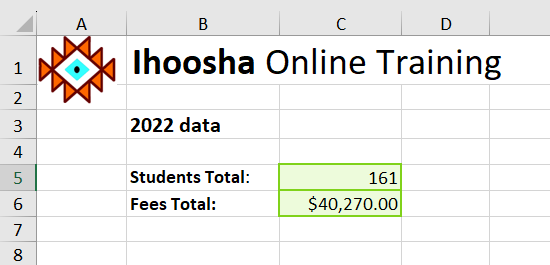
MedAttrib: author-generated. MS Excel data-linking process from an external file.