Chapter 7: Data Ranges

What We’ll Cover >>>

• Datasets
• Data Ranges
• Named Ranges
• Moving Ranges
• Sorting Data
• Filtering Data

Datasets

Excel is all about data. The data is for viewing, organizing, sorting/filtering, analyzing, and calculating so that business problems can be considered and solved. The more organized the data is, the better you will be able to use it, analyze it, and get the needed calculations, graphs, and pivot tables to answer your questions.

A dataset is a range of contiguous cells on an Excel worksheet, which contain data to analyze. In a worksheet, cells with data on a spreadsheet would be a data set. However, a dataset doesn’t really mean anything until you determine what it exists for and what kind of analysis needs to happen.

ACTION: Quick Task

Let’s look at an image of some Excel work. In it the cells A1 through D7 have data that seems related to each other. Cells E1-E6 is a column of data, as is the column of G1-G5. This is all part of a dataset, although only cells A1 – C7 seem to meet the dataset definition of being contiguous.

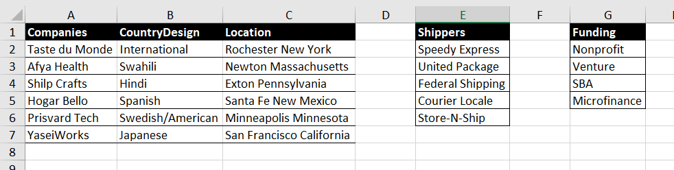
MedAttrib: author-generated. MS Excel dataset.

Data Ranges

The phrase data range tends to be a statistical term to refer to the spread of data from the lowest to the highest value in the distribution. However, Excel refers to named data sets as a named range, so for the purposes of this textbook, we will refer to dataset and data range (in nonstatistical analysis) as the same thing. As a reference to data in a sheet or a table, range of data is simply a set of data, a designated range of cells in tabular format. A whole spreadsheet would be a dataset; a data range would be a group of cells that are being specifically worked with.

• Cell contents: As discussed before, all data in Excel (other than inserted objects like pictures) is input into cells. Each cell is something that, as part of a row and column, can be sorted, calculated, and tell a story.
• Cell addresses: Data are entered and managed in cells by entering numeric and non-numeric data. Each cell in an Excel worksheet contains an identification address, which is defined by a column letter followed by a row number. For example, the top left cell A1. This would be referred to as cell location A1 (or cell reference A1). You can navigate in an Excel worksheet with your mouse pointer or using the arrow buttons on your keyboard.
• Column Headings: In Excel, data rarely means anything to a viewer if there is no context attached to it. Commonly this is done through column headings, which identify what the content in the column is supposed to be. This can also be done as row headers instead, but in this course we’ll mostly use the standard column headings.
• Rows and columns: These make up the range of data in a dataset, with or without column headings.

Data range activities

A range of data in a dataset can be:

• Resized: You can resize columns from the Home tab Cells group to reveal information that looks cut off, or to narrow them if there is too much space. Same with rows if the row is too tall or seems to have cut off anything other than the first line of text.
• Inserted/Deleted: Rows and columns can be inserted as needed from the Home tab Cells group, in order to expand for data to be added. Existing columns and rows can also be deleted.
• Hide/Unhide: You may have a worksheet with a lot of columns, but really only need to see some of the data to decision. Hiding columns or rows can help you focus.
• Sorted: In addition, information in a range of data can be sorted from the Data tab Sorts & Filters group, so that one or more column)s) shows information in an alphanumeric order or in some more customized order.
• Filtered: A range of data may have information about more customers or other content than you need: using a filter from the Data tab Sorts & Filters group lets you temporarily hide unwanted information so you can get a snapshot view.
• Freezing Panes: If a range of data is made up of hundreds of records – long enough that you need to scroll down several pages to see it all, or over enough columns that you can’t see the important left-most columns, you can freeze a column or two, or the header row, so that the information remains in view no matter how much you have to scroll.

ACTION: Quick Task

Back to the image again:

MedAttrib: author-generated. MS Excel dataset.

In here, all three batches of data are ‘ranges’ of data. This is important, because we may want to actually reference them in a tidy way for formulas and general reference. As they exist now, they are simply designated by the cell collections. A1:C7, E1-E6, G1-G5.

Named Ranges

As noted above, a range of data is simply a dataset that can and will have work done with it. However, what needs to happen with data is what is important. Formulas that calculate data for specific purposes need to be able to find the data and easily add it to the formula. Sometimes the data will be all the contents of a table. Sometimes it will be only a column or two, or a few rows in a larger data range. In these cases, being able to “set aside” the data range in an identifiable way can make writing and fixing formulas easier. You can do this by identifying/naming data ranges.

• Selecting: You select a data range by choosing a selection of row and column cells, such as dragging your cursor to select A1 through D10, or typing A1:D10.
• Naming: To make that data range useful and easy to refer to in a formula, you need to name it. This can be done in the Formulas tab’s Defined Names group by using the Name Manager panel to give the data range a name. Once this is done, you can see a list of every named data range in the Excel Address field.
• Use in formulas: In a formula, you can use the named range as the data range reference in the formula, such as =SUM(Totals)

ACTION: Try Me activity

Let’s now work with an Excel file: Ch7-DataRanges.xlsx. This is a dataset from our friend Taste du Monde that we can use for looking at a dataset, identify ranges of data, and set names for two or three of them.

Save a copy of Ch7-DataRanges.xlsx to your Examples folder, then open it for work. It already includes the Taste du Monde logo icon and WordArt and link to their website. It also includes records of customer data including names, addresses, emails, and opt-in decisions.

The whole set of A6 through J36 is a data set – a range of data / data range.

• Select only cells A6 – C36. This is a range of data of that range of cells of customer first and last names and their customer IDs.
• Deselect it.
• Select only cells A6 through J9. This is a range of data of the first three customer records and the header row.
• Deselect it.

Now, let’s choose a range of data and name it for possible later use.

• Select only cells F6 – H36.
• With these cells selected, choose the Formulas menu tab/ribbon.
• In the Formulas ribbon, look at the Defined names group. Select the dropdown arrow of the Defined Name button.
• Click on “Defined name”, which will open a dialog box.
• In the dialog box, in the Name field, type TM_Region.
• In the dialog’s Scope, leave the default of workbook.
• In the comment field, type: Taste du Monde customer regions.
• In the Refers to field, note that Excel recognizes that you selected =Customers!$F$6:$H$36, which is referring to the worksheet called Customers, and the range of data from F6 – H36.
• Click OK.
• Now, click on the dropdown arrow of the Name field in the Excel UI (above cell A1), which usually shows the address of the Cell you have clicked in. When you click on the arrow, you should see TM_Region listed. This is a named data range.
• Click on TM_Region in that Name field. Excel will select the range of data you just named – cells F6 – H36 – for you.
• SAVE your work as you go: Keybind is CTRL S / Mac CMD S.

Let’s practice another one.

• Select the range of cells from I6 – J36.
• With the selection active, go to the Formulas ribbon, Defined Names group, and select the Name Manager icon. This will open a panel which already lists the TM_Region named data range we already created.
• In this panel, click the button New. In the Name, type TM_OptIn. In the comment, type Taste du Monde newsletter opt-in.
• Look at the data range given: =Customers!$I$6:$J$36.
• Click OK. You should now see both named ranges listed in the Name Manager panel.
• Click OK again to exit the panel.
• SAVE your work as you go: Keybind is CTRL S / Mac CMD S.

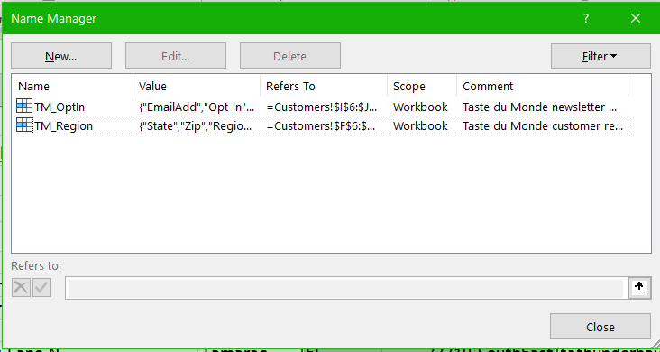
MedAttrib: author-generated. MS Excel Name Manager panel.

Editing Ranges

Next, we’ll find out what happens when we delete some data from a named range.

• With the Ch7-DataRanges.xlsx file still open, select Column G and delete it.
• In the Name field above cell A1, click on the named range TM_Region. Excel now should select only the range F6-G36. The G column now contains the data from the Region, since the zip code data has been deleted. It seems as if Excel has no issue with the deletion of a column that was in the named range.
• In the Formula ribbon, Defined Names group, select the Name Manager icon.
• In the Name Manager panel, double-click the TM_Region range. Look at the “Refers to”, which now reads =Customers!$F$6:$G$36.
• Click Cancel to exit TM_Region.
• Double-click on TM_Optin, and look at the “Refers to”, which now reads =Customers!$H$6:$I$36. This happened because a column was removed from the worksheet, and Excel adapted by adjusting even the TM_OptIn selection for the named data range.
• Cancel out of that, and cancel out of the Name Manager panel.
• SAVE your work as you go: Keybind is CTRL S / Mac CMD S.

Moving Ranges

Let’s move a named range.

• If you have not yet saved Ch7-DataRanges.xlsx, DO IT NOW, please. We will do a task we may not want to keep but you don’t want to lose any previous work.
• With Ch7-DataRanges.xlsx still open, use the Name field above cell A1 to choose TM_OptIn. Excel will select the cells that make up that named range.
• Right-click and choose Cut (or use the shortcut of CTRL X / CMD X for Mac), which will ‘cut’ the selection.
• Place your cursor in cell L6, right-click, and choose Paste (or CTRL V / CMD V).
• The named range has been moved. This is just demonstration, which we are not keeping.
• Close the Ch7-DataRanges.xlsx without saving it.

Sorting Data

Let’s work with sorting and filtering data ranges. We actually do want to work with the Ch7-DataRanges.xlsx file again. We just didn’t want to save the last set of changes made. Please open the Ch7-DataRanges.xlsx file.

The dataset has a header row, which has been emphasized with bold text. This will help us identify what we want to sort and filter.

The important thing to know about datasets and named data ranges is that, although they display data in columns and rows, the data is not actually connected. Let’s see what this means.

• Select the contents of column I, cells I6-I36. Copy it, then move your cursor to Cell J6.
• In cell J6, paste the data you just copied. Now you have two columns of Opt-In responses.
• Select the data of column J’s cells J6-J36. Use the fill color paintbucket in the Home ribbon to paint the cell backgrounds a light color, like gray.
• With this J column J6-J36 data still selected, choose the Data tab ribbon. In the ribbon, choose the Sort & Filter group, Sort A to Z button.
• You should see a sort warning message:

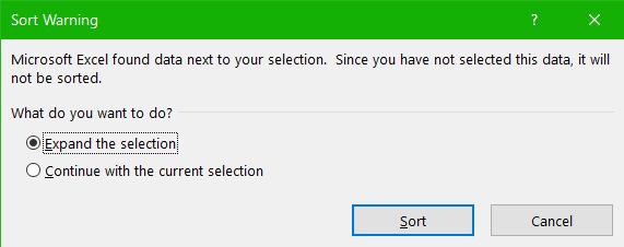
MedAttrib: author-generated. MS Excel Sort warning.

• What to do? Let’s choose “Continue with the current selection” then click the Sort button to observe what happens.
• Review the two Opt-In columns. The J column one is out of order compared to the original I column. That is a problem.

Why did we go through this? Well, back in the Bronze Age when the author first worked with Excel, there were no warnings about sorts of data in relation to a dataset that wasn’t actually connected as an Excel table object. The author hangs her head in shame at the data sorting mistakes that occurred. Now, even with the Excel sort warning, it can still be easy for an inexperienced data analyst to accidentally sort only part of a dataset, which would corrupt a batch of data when some information becomes untethered from its proper record. This would affect the data accuracy, the results of pivot summary tables, and definitely skew charts based on the data.

Let’s be more careful and try again.

• First, delete all of column J – the incorrectly sorted column. column J will now be blank and unformatted again.
• Next, select data from column C, cells C6-C36. This will give us the last names of customers.
• With this selection, again go to the Data ribbon, and select the Sort icon.
• Again, we will get the Sort warning. In this case, leave the default selected response of “Expand the selection”, then click the Sort button.
• Now, Excel will select – for us – the entire contiguous range of data from cell A6 through I36.
• In addition, the Sort panel gives us a choice of what to sort. In the Column Sort By field, choose CustLName.
• In the Sort By field, leave the default of Cell Values – Excel will sort based on the content rather than some other method.
• In to Order field, keep the default of A to Z.
• Click the OK button to generate the sort.

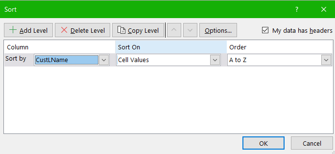
MedAttrib: author-generated. MS Excel Sort panel.

The whole data range of Cells A6-I36 should have been properly sorted, in A-Z order, based on the customer’s last name.

• SAVE your work as you go: Keybind is CTRL S / Mac CMD S.

Filtering Data

Can we also filter data in a data range? Filtering allows you to hide items in a column based on some reason you have to exclude it. Let’s find out.

• Place your cursor on any cell in the data range of cells A6-I36.
• Choose the Data ribbon Sort & Filter group, and select the Advanced Filter button.
• An Advanced Filter panel opens, which Excel already displays the List range of A6-I36 because the program “sees” a contiguous range of data that seems related. That is efficient. So is the default option to filter the list in place. However, the filter requires some Criteria range to filter in or out things for specific reasons. That requires us to give a specific data range – like one of the columns.

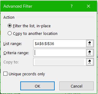
MedAttrib: author-generated. MS Excel Advanced Filter panel.

• Click inside the Criteria range field, then type F6:F36. This should select the State column’s contents in our dataset. Then click OK.

Hmmmm. Looks like nothing happened. Why? Well, in the end, we asked for a filter, yet the advanced filter didn’t really know what to filter for, and given that we were working with an unconnected dataset of rows and columns, Excel couldn’t comply. Let’s try something else.

• Place your cursor on any cell in the data range of Cells A6-I36.
• Choose the Data ribbon Sort & Filter group, and select the larger Filter icon. Something interesting happens. In the header row of our dataset, a bunch of small dropdown arrows appears. This tethers together the columns and rows, so that a filter can work with the range of A6-I36.
• Click the dropdown arrow in cell F6.
• When you look at the filter arrow’s dropdown, you can see that the column can actually be SORTED, like a basic alphabetical sort. Yay! Let’s click the Sort A to Z.
• Nice! Even by clicking A-Z in F6, the whole dataset sorts to the A to Z of the States. Now, let’s filter out all states but California (CA).
• Click the dropdown arrow in Cell F6. In the dropdown, Uncheck the Select all box. Then, put a checkmark only in the CA checkbox, and click OK.
• There we have it; the dataset has had every state (and the related state’s records) filtered out except for those of California (CA). All the data still exists, but we can review only these two records until we clear the filter.
• To clear the filter, click the dropdown arrow in Cell F6. In the dropdown, choose the Clear Filter from “State”.
• SAVE your work as you go: Keybind is CTRL S / Mac CMD S.
• Close your saved file – we are finished.

Here is the really great news. As easy as all this is, in the next chapter, we will work with Excel table objects, so that we can utilize Excel’s connecting of data in a range without having to go through some of these manual steps.

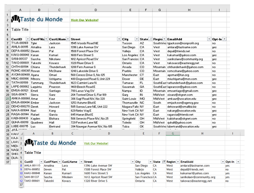
MedAttrib: author-generated. MS Excel unfiltered and filtered dataset.